Download
1 / 12
120 likes | 464 Views
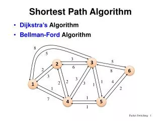
CS 155, Programming Paradigms Fall 2014, SJSU the Bellman-Ford shortest path algorithm. Jeff Smith. Shortest paths in directed graphs. It’s common to ask for the shortest path from vertex v to vertex w in a weighted digraph.

E N D
CS 155, Programming ParadigmsFall 2014, SJSUthe Bellman-Ford shortest path algorithm Jeff Smith
Shortest paths in directed graphs • It’s common to ask for the shortest path from vertex v to vertex w in a weighted digraph. • From studying Dijkstra’s (and perhaps Floyd’s) algorithm, you should remember that • conventionally, “shortest” means “cheapest” • the cost of a path is the sum of its edge costs • if there’s a directed cycle of negative cost, then there can be no cheapest path • other directed cycles can be omitted
Limitations of Dijkstra’s algorithm • Dijkstra’s algorithm is reasonably efficient in the single-source case • but assumes that no edge cost is negative • and thus that there are no negative-cost cycles reachable from the source • Recall that it’s based on the notion of relaxation • and isn’t quite greedy or dynamic programming • we discuss relaxation below
Dealing with the limitations of Dijkstra’s algorithm • The Bellman-Ford algorithm will determine whether such a negative-cost cycle exists • If so, it will fail • in Java, we can return null, or throw an exception • If not, it will return a structure giving the lowest cost to each vertex • and enough information to reconstruct the path
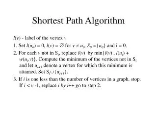
The Bellman-Ford algorithm • The Bellman-Ford algorithm repeatedly visits each edge of the graph • asking whether relaxation at the edge can shorten any paths from the source vertex s • and recording the shortening if so • The only other steps initialize each vertex, and check for reachable negative-cost cycles • as seen in the code of p. 651, CLRS • The algorithm isn’t obviously correct.
Relaxation • Let x.d (as in CLRS) be the lowest known cost of reaching x from the source vertex s • Relaxation of an edge (u,v) • asks whether v.d can be lowered by adding (u,v) to the end of the path to u of cost u.d • if so, updates v.d accordingly • and records that u is the predecessor v.π of v on v’s new cheapest path
Initialization in Bellman-Ford • Initially, • the cheapest path to s has cost 0 • the cheapest path to any other vertex v has cost ∞ • no vertex has a predecessor on the path to it • So initialization takes time proportional to the number |V| of vertices.
Lengths of shortest paths • A simple observation, hinted at above, will simplify the computation. • Namely, if there are no reachable negative-cost cycles, no cheapest path can have a repeated vertex • if it repeated vertex v, then the cycle between the two occurrences of v could be omitted • and the new path would be at least as cheap • So no cheapest path can be longer than |V|.
Time complexity • Since no shortest path can have length greater than |V|, the main loop of the algorithm is iterated Θ(|V|) times • And each iteration takes time Θ(|E|) • where E is the set of edges • and each edge has to be relaxed in each iteration • So the overall time complexity is Θ(|V||E|) • since the final check for reachable negative-cost cycles takes time Θ(|E|)
An example of the algorithm • Let s=1 in the graph of p.690, CLRS. • Then the initial value of d is [0, ∞, ∞, ∞, ∞] • After the first three iterations, the values are • [0,31,-14,25,-41], [0,31,-34,25,-41], [0,13,-34,25,-41] • here edges are relaxed in row-major order • and subscripts represent π values • There’s no change in later iterations, so the final value is [0,13,-34,25,-41] • cf. the top row of L(4), p. 690, or D(5) & Π(5), p. 696
Correctness of Bellman-Ford • Claim: after iteration k of the main loop, all shortest paths of length k have been found. • The claim is true for k=0, so by way of proof, let i be the minimal counterexample, and (vi-1,vi) the final edge of the shortest path. • By minimality, the shortest path vi-1 is found during or before iteration i-1. • But then iteration i will correctly find (vi-1,vi).
End of the correctness proof • From our claim, all shortest paths have been found of length n after the last iteration • If there are no reachable negative-cost cycles, these paths include all shortest paths • and the loop of lines 5-7 will not return false • If there are, then by the algebra of pp. 653-4, some relaxation of this loop returns false • intuitively, each loop iteration reduces v.d for some v in the cycle, once the cycle has been traversed – which must happen by iteration |V|