
Chapter 3: Random Variables and Probability Distributions
E N D
Presentation Transcript
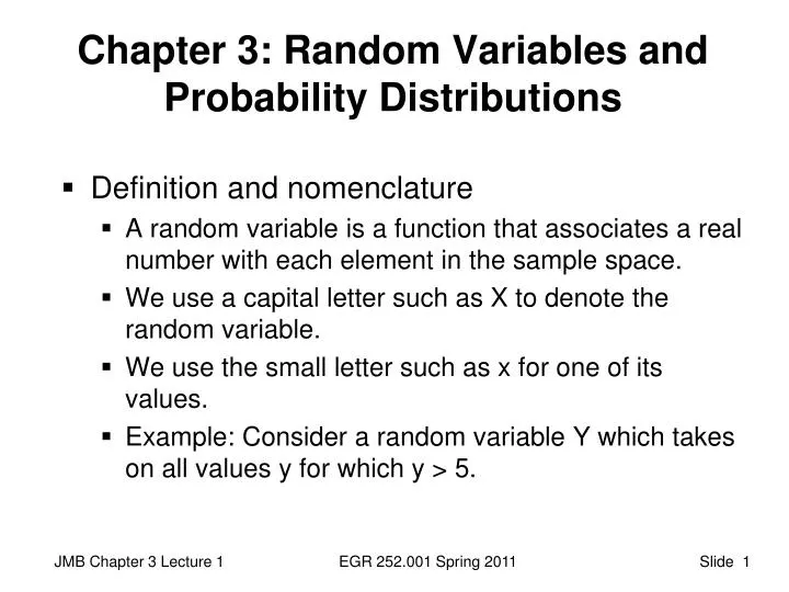
Chapter 3: Random Variables and Probability Distributions • Definition and nomenclature • A random variable is a function that associates a real number with each element in the sample space. • We use a capital letter such as X to denote the random variable. • We use the small letter such as x for one of its values. • Example: Consider a random variable Y which takes on all values y for which y > 5. EGR 252.001 Spring 2011
Defining Probabilities: Random Variables • Examples: • Out of 100 heart catheterization procedures performed at a local hospital each year, the probability that more than five of them will result in complications is P(X > 5) • Drywall anchors are sold in packs of 50 at the local hardware store. The probability that no more than 3 will be defective is P(Y < 3) EGR 252.001 Spring 2011
Discrete Random Variables • Problem 2.53 Page 55 Modified • Assume someone spends $75 to buy 3 envelopes. The sample space describing the presence of $10 bills (H) vs bills that are not $10 (N) is: • S = {NNN, NNH, NHN, HNN, NHH, HNH, HHN, HHH} • The random variable associated with this situation, X, reflects the outcome of the experiment • X is the number of envelopes that contain $10 • X = {0, 1, 2, 3} EGR 252.001 Spring 2011
Discrete Probability Distributions 1 • The probability that the envelope contains a $10 bill is 275/500 or .55 • What is the probability that there are no $10 bills in the group? P(X = 0) =(1-0.55) * (1-0.55) *(1-0.55) = 0.091125 P(X = 1) = 3 * (0.55)*(1-0.55)* (1-0.55) = 0.334125 • Why 3 for the X = 1 case? • Three items in the sample space for X = 1 • NNH NHN HNN EGR 252.001 Spring 2011
Discrete Probability Distributions 2 P(X = 0) =(1-0.55) * (1-0.55) *(1-0.55) = 0.091125 P(X = 1) = 3*(0.55)*(1-0.55)* (1-0.55) = 0.334125 P(X = 2) = 3*(0.55^2*(1-0.55)) = 0.408375 P(X = 3) = 0.55^3 = 0.166375 • The probability distribution associated with the number of $10 bills is given by: EGR 252.001 Spring 2011
Example 3.8, pg 80 • Shipment: 8 computers of which 3 are defective • Random purchase of 2 computers • What is the probability distribution for the random variable X = defective computers purchased? Possibilities: X = 0 X =1 X = 2 Let’s start with P(X=0) P = specified target / all possible (0 defectives and 2 nondefectives are selected) (all ways to get 0 out of 3 defectives) ∩ (all ways to get 2 out of 5 nondefectives) (all ways to choose 2 out of 8 computers) (all ways to choose 2 out of 8 computers) EGR 252.001 Spring 2011
Discrete Probability Distributions • The discrete probability distribution function (pdf) • f(x) = P(X = x) ≥ 0 • Σxf(x) = 1 • The cumulative distribution,F(x) • F(x) = P(X ≤ x) = Σt ≤ xf(t) • Note the importance of case: F not same as f EGR 252.001 Spring 2011
Probability Distributions • From our example, the probability that no more than 2 of the envelopes contain $10 bills is • P(X ≤ 2) = F (2) = _________________ • F(2) = f(0) + f(1) + f(2) = .833625 • (OR 1 - f(3)) • The probability that no fewer than 2 envelopes contain $10 bills is • P(X ≥ 2) = 1 - P(X ≤ 1) = 1 – F (1) = ________ • 1 – F(1) = 1 – (f(0) + f(1)) = 1 - .425 = .575 • (OR f(2) + f(3)) EGR 252.001 Spring 2011
Another View • The probability histogram EGR 252.001 Spring 2011
Your Turn … • The output of the same type of circuit board from two assembly lines is mixed into one storage tray. In a tray of 10 circuit boards, 6 are from line A and 4 from line B. If the inspector chooses 2 boards from the tray, show the probability distribution function associated with the selected boards being from line A. EGR 252.001 Spring 2011
Continuous Probability Distributions • The probability that the average daily temperature in Georgia during the month of August falls between 90 and 95 degrees is • The probability that a given part will fail before 1000 hours of use is In general, EGR 252.001 Spring 2011
Visualizing Continuous Distributions • The probability that the average daily temperature in Georgia during the month of August falls between 90 and 95 degrees is • The probability that a given part will fail before 1000 hours of use is EGR 252.001 Spring 2011
Continuous Probability Calculations • The continuous probability density function (pdf) f(x) ≥ 0, for all x ∈R • The cumulative distribution,F(x) EGR 252.001 Spring 2011
Example: Problem 3.7, pg. 88 The total number of hours, measured in units of 100 hours x, 0 < x < 1 f(x) = 2-x, 1 ≤ x < 2 0, elsewhere • P(X < 120 hours) = P(X < 1.2) = P(X < 1) + P (1 < X < 1.2) NOTE: You will need to integrate two different functions over two different ranges. b) P(50 hours < X < 100 hours) = Which function(s) will be used? { EGR 252.001 Spring 2011