Download
1 / 16
160 likes | 258 Views
Suggested readings. Historical notes Chap1 , Andrieu , C., et al. (2003). An Introduction to MCMC for Machine Learning. Machine Learning, 50, 5–43 . Section 11.11 by Gelman . Markov chains

E N D
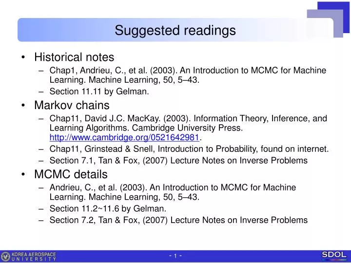
Suggested readings • Historical notes • Chap1, Andrieu, C., et al. (2003). An Introduction to MCMC for Machine Learning. Machine Learning, 50, 5–43. • Section 11.11 by Gelman. • Markov chains • Chap11, David J.C. MacKay. (2003). Information Theory, Inference, and Learning Algorithms. Cambridge University Press. http://www.cambridge.org/0521642981. • Chap11, Grinstead& Snell, Introduction to Probability, found on internet. • Section 7.1, Tan & Fox, (2007) Lecture Notes on Inverse Problems • MCMC details • Andrieu, C., et al. (2003). An Introduction to MCMC for Machine Learning. Machine Learning, 50, 5–43. • Section 11.2~11.6 by Gelman. • Section 7.2, Tan & Fox, (2007) Lecture Notes on Inverse Problems
Markov Chain • Weather in the land of Oz • Land of Oz has unique weather system. Note that next day state is not affected by the previous states. • Case study • It is R today. What is the probability of S tomorrow ? • What is the probability of S, day after tomorrow ? • For i’th state, what is the probability of j’th state, day after tomorrow ? • After many days like 100 days ? • Let the initial state is always R. Calculate states after 3, 10, 100 days.Let the initial state has equal chance. Calculate states after 3, 10, 100 days. If N, likely to S and R the next day, not N again. If R or S, 50% of the same the next day. If changed, only half of this change to N.
Markov Chain • Remarks • For a set of states S={s1,s2,…,sr}, Markov chain is a process that a new state sj is determined by current state siwith probability pij. Note that the new state is not affected by the previous states. • pij is called transition probabilities, denoted as P(j|i) = pij.The row vector, called probability vector (or distribution), sums to 1.pij(n) of the matrix Pn gives the probability that we have state sj, starting from state si, after n steps. • As n→∞, Pn approaches limiting matrix W with all rows the same vector w. w is obtained by using wP=w or w(P-I)=0. in fact, w is left eigenvector of matrix P. • Let u be arbitrary starting dist. Then probability distribution after n →∞ steps is uPn = w, which means that regardless of initial u, one gets always the same distribution w after many steps.
Markov Chain Monte Carlo • Introduction • MCMC is a strategy for generating samples x(i) by exploring the states using a Markov chain mechanism, such that the samples x(i) mimic samples drawn from the target distribution p(x). • MCMC is used when it is not possible (or not computationally efficient) to sample qdirectly from p(q|y). Instead, sample iteratively such that at each step of the process we expect to draw from a distribution that becomes closer and closer to p(q|y). • MCMC doesn’t require that p(q|y) be normalized. • For a wide class of problems, this appears to be the easiest way to get reliable results.
Markov Chain Monte Carlo • Forward process: Markov process • Stochastic process x(i) is called Markov chain if • Given a transition matrix T, find equilibrium distribution p. • Example: • Inverse process: MCMC process • Given a distribution p, construct transition matrix T of Markov chain. Then we obtain after Markov process, the target distribution p. • Example:
Df • In Markov simulation, sequences of simulation draws are created; each sequence is produced by starting at an arbitrary point , and drawing from a transition distribution . The transition probability distribution should be constructed so that the Markov chain converges to a stationary distribution which is the target of our concern. • Recent survey places the Metropolis algorithm as one of the greatest ten algorithms of science and engineering development of 20th century. The algorithm is playing key role in sampling method known as MCMC. These algorithms have played a significant role in statistics, econometrics, physics and computing science over the last two decades.
Metropolis-Hastings algorithm • Introduction • Most popular MCMC method. Other MCMC algorithms are interpreted as special cases or extensions of this algorithm. • MH Algorithm • A proposal distribution q(x*|x) is introduced. • The MH step is to sample a new candidate x* given the current x based on q(x*|x). Then the point is accepted with probability Otherwise it remains at x. • By repeating this steps, one obtains in the end the samples of p(x).
Metropolis-Hastings algorithm • Metropolis algorithm • A proposal distribution q(x*|x) is symmetric w.r.t x* and x. Then the ratio is simplified. Example: normal pdf at x* with mean at x equals to the vice versa. • Practice with matlab • Generate samples of this distribution using a proposal pdf • As the random walk progresses, the number of samples are increased, and the distribution converges to the target distribution.
Metropolis-Hastings algorithm • Notes • MH requires careful design of the proposal distribution • Allowing asymmetric jump rules can increase the speed of random walk. • There is matlab function for MH algorithm. • mhsample(1,N,'pdf',p,'proprnd',qrnd,'proppdf',q); • Variants of MCMC are • Hybrid Monte Carlo • Slice sampling • Reversible jump MCMC
Simulated annealing for global optimization • Algorithm • Target distribution is objective function in optimization problem. After sampling via MH algorithm, the optimum solution is obtained as the mode of the simulated distribution, i.e., • Using just original function is inefficient. Simulated annealing was developed to enhance speed of finding this, in which pdf value at iteration i is replaced by where Ti is decreasing cooling schedule • Thus SA is just a minor modification of standard MCMC algorithms.
Simulated annealing for global optimization • Algorithm
Gibbs sampler • Algorithm • Particular Markov chain useful for multidimensional problems, also called alternatingconditionalsampling. • Let x=(x1,x2,…,xn). Each iteration of the Gibbs sampler cycles through the components, drawing each parameter conditional on the values of all the others. There are thus n steps in an iteration. • Each parameter xj is updated conditional on the latest values of the other components which are • the iteration i values for the already updated components and • the iteration i-1values for the others not updated yet.
Gibbs sampler • Practice with matlab • Generate samples of bivariatenormal distribution with correlation r. • To apply Gibbs, we need conditional distributions, using the properties of multivariate normal distribution ((A.1) or (A.2) on page 579) • Gibbs sampling where sample for conditional pdf drawn by matlabfunction. • Gibbs sampling where sample for conditional pdf drawn by MH algorithm.
MH Algorithm for two parameters • Remark • Gibbs sampler samples alternatively for each component of the parameter vector while MH algorithm samples altogether for the parameter vector. • Algorithm • is outlined via example.
Inference and convergence • Remarks • If iterations not proceeded long enough, result can be erroneous. • Recommended simulation is to employ multiple sequences with starting points dispersed over the domain. Then monitor the variation between and within the sequence and proceed until the within variation equals the between variation. More detail is addressed in the textbook p296. • Early iterations should be discarded. Usually the first half of each sequence is discarded. This discarding activity is referred as ‘burn-in’. • One can apply several graphical and statistical tests to assess, roughly, if the chain has stabilized. In general, none of these tests provide entirely satisfactory diagnostics. • See another comment on the convergence at Chap. 29 Monte Carlo Methods in David J.C. MacKay. (2003). Information Theory, Inference, and Learning Algorithms. Cambridge University Press.
Homework • Problem • For the 3.7 Example: Bioassay experiment, • Perform Metropolis algorithm of two parameters to obtain samples of the posterior distribution. • Draw scatter plot. • Draw traces of each parameters and sequence of points in 2-D domain. • Compute mean, 95% conf. intervals, variances and correlation of the two parameters. • Try different initial point, different proposal density and compare the results 4.