Download
1 / 48
480 likes | 581 Views
Cooperative cost sensitive IP Routing (Authors: Dean H.Lorenz Ariel Orda Danny Raz Yuval Shavitt). Presenting : Vadim Drabkin. A Short Introduction to IP Routing. Every host interface has it’s own IP address 5 address classes(A,B,C,D(multicast),E(reserved) Interior routing protocols

E N D
Cooperative cost sensitive IP Routing(Authors: Dean H.Lorenz Ariel Orda Danny Raz Yuval Shavitt) Presenting : Vadim Drabkin Seminar in Packet Networks
A Short Introduction to IP Routing • Every host interface has it’s own IP address • 5 address classes(A,B,C,D(multicast),E(reserved) • Interior routing protocols • Distance-vector routing and RIP • Link state routing and OSPF • How does a host perform routing Seminar in Packet Networks
IP packet format Seminar in Packet Networks
IP packet format (cont.) • Header Length (because of the options field) • Total length includes header and data • Service Type – lets user identify his needs in terms of bandwidth and delay (for example QoS) • Time to Leave prevents a packet from looping forever • Protocol, indicates the sending protocol (TCP,UDP,IP…) • Source Address • Destination Address Seminar in Packet Networks
Unicast Routing • We need to know the next hop to reach a particular network number (can be done with a routing table) • The routing table is a simple database held by every router. It tells the router how to forward packets whose destination IP address is not equal to router IP address. • Theoretically ,the routing table needs an entry for every network in the Internet. Practically, most of the networks are mapped into a single “default” entry. Seminar in Packet Networks
An Autonomous System (AS) • A region of the Internet that is under the administrative control of a single entity and has a single routing policy. • The routing problem is divided into : • Routing within a single AS (intra domain routing) • Routing between AS (inter domain routing) • An AS can run whatever intra-domain routing protocols it chooses Seminar in Packet Networks
Internet routing protocols • Interior routing protocols : • RIP (routing information protocol) • A distance vector algorithm • OSPF (open shortest path first) • A link state algorithm • IS-IS – a link state protocol and quite similar to OSPF • Exterior routing protocols • EGP • BGP (border gateway protocol), based on path vectors than on distance vectors Seminar in Packet Networks
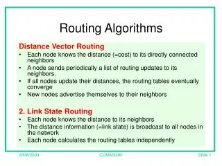
Distance Vector routing • A node tells its neighbors it’s best idea of distance to every other node in the network • Node receives these distance vectors from it’s neighbors • Node then updates its notion of the cost of the best path to each destination, and the next hop for this destination • A distributed implementation of the Bellman-Ford algorithm Seminar in Packet Networks
Distance Vector routing (cont.) • RIP is simple for implementation but is inadequate for larger and complex autonomous systems because of the long convergence following failures. • RIP is being replaced by OSPF (Open Shortest Path First), which uses link-state rather then distance-vector routing. Seminar in Packet Networks
Link-state routing • Each router creates a set of link-state packets (LSPs) that describe it’s links • Each LSP is distributed to every router using a controlled flooding algorithm. • Each router can independently compute optimal paths to every destination. Seminar in Packet Networks
The advantages of link-state over distance vector • Fast, loopless convergence • Can support routing according to different metrics • Each link is associated with a value for each metric • A routing table is computed for every metric • A Link-state protocol, the preferred choice for interior routing • OSPF version 2 is defined in RFC-2328 Seminar in Packet Networks
Introduction • In the traditional IP scheme both the packet forwarding and routing protocols (RIP and OSPF) are source invariant i.e., their decisions depend solely on the destination IP address • Recent protocols allow routing and forwarding decisions to depend on both the source and destination addresses • The benefit of the per-flow forwarding is well accepted as well as the practical complication of its deployment. Seminar in Packet Networks
Introduction (cont.) • In particular any solution that requires to consider some quadratic number of source-destination pairs (rather than a linear number of destinations) is far from being scalable. • This work aims at investigating the performance gap between source invariant and per-flow schemes. • Facing the gap between the two basic schemes, in this study we propose a novel source invariant scheme. Seminar in Packet Networks
Introduction (cont.) • The scheme exhibits a significantly improved performance over the standard source invariant scheme, and comes close to the performance of per-flow schemes. • At the same time it maintains the practical advantage of independence of source addresses. • But it requires a higher degree of centralization. • However increased centralization is one of the processes that can be observed in the evolution of the Internet. Seminar in Packet Networks
Main Contributions • We show that theoretically any routing algorithm based on static weights can perform as bad as any source invariant scheme • We show that the gap in performance between IP routing and OSPF may be as bad as (N is a number of nodes in the network) • OSPF is worse than per flow routing Seminar in Packet Networks
Main Contributions (cont.) • Thus, we present a family of centralized algorithms that set forwarding tables in IP networks, based on dynamically changing weights. • The centralized algorithm input is the network topology and a flow demand matrix that based on long term traffic statistics. Seminar in Packet Networks
Model and Problem Formulation • The network is defined as a graph G(V,E), V = |n|, E = |m|. Each link has a capacity Ce,Ce>0. A demand matrix, D={Di,j}, defines the demand Di,j, between each source i and destination j. • We define the following routing paradigms : • Unrestricted Splitable Routing (US-R) – a flow can be split among the outgoing links arbitrarily • Restricted Splitable Routing (RS-R) - a flow can be split over a predefined number L of outgoing links • RS-R1 – a special case of RS-R, when L = 1, which is known as the unsplitable flow problem. Seminar in Packet Networks
Model and Problem Formulation (cont.) • A routing assignment is a function R:V^4->[0..1], such that Fu,v(i,j) (i=source,j=destination) is the relative amount of (i,j) flow that is routed from a node u to neighbor v • A routing is called source invariant if : Fu,v(i1,j)=Fu,v(i2,j)= Fu,v(j) (flow amount depends on destination j only) • Standard IP Forwarding Routing (IP-R) – The special case of source invariant RS-R1 , for each u and j belongs to V, exists v and Fu,v(j) = 1 Seminar in Packet Networks
Model and Problem Formulation (cont.) • OSPF routing (OSPF-R) – A class of source invariant routing assignments that split flow evenly among next hops. • We denote Ď =Ď(G,D,R) the allocation matrix that results from the application of the rule (for example max-min fairness) on network G,demand matrix D and routing assignment R. The throughput of the matrix is the sum of its components. Seminar in Packet Networks
Model and Problem Formulation (cont.) • Link congestion factor is the ratio between the flow routed over the link and its capacity; the network congestion factor is the largest link congestion factor. • For a network G,routing assignment R and demand matrix D are said to be feasible if the resulting congestion factor is at most 1 Seminar in Packet Networks
Optimization Problems • Problem Congestion Factor – Given a routing paradigm, a network G(V,E) with link capacities and a demand matrix D, find a routing assignment R that minimizes the network congestion factor. • Problem Max Flow - Given a routing paradigm, a network G(V,E) with link capacities and a demand matrix D, find a routing assignment R such that allocation matrix Ď(G,D,R) has maximum throughput. Seminar in Packet Networks
Hardness Results • Finding an optimal IP routing(Problem Congestion factor with IP-R) is NP-hard even for a single destination. • Theorem 1 : The decision optimal IP routing problem is at least as hard as the subset sum problem. (The subset problem is defined as follows: given ai, i=1,…,n elements with sizes s(ai) belongs to Z+ and a positive integer B, find a subset of the elements whose size sum equals to B. ) Seminar in Packet Networks
Hardness Results (cont.) • Proof: we build the reduction from subset problem to IP routing decision problem • Because subset sum problem is NP-hard , we conclude that the decision optimal IP routing problem is NP-hard as well. • Every node i creates a flow |i| to destination and the question is how to route the flow (to x or to y) to destination Seminar in Packet Networks
Theoretical Bounds • In this section we study the differences among the routing paradigms by showing upper and lower bounds on the worst case ratio between the performance of these paradigms. • IP-R vs RS-R1 and OSPF-R • We show that IP-R can be than RS-R1 and OSPF-R with respect to both optimization criteria. Seminar in Packet Networks
IP-R vs RS-R1 and OSPF-R • All link capacities are 1. Every node creates a flow 1 to destination. Seminar in Packet Networks
IP-R vs RS-R1 and OSPF-R IP-R Network congestion factor is N 1 IP-R throughput is 1 1 1 Seminar in Packet Networks
IP-R vs RS-R1 and OSPF-R RS-R1 1 RS-R1 throughput is N RS-R1 Network congestion factor is 1 1 1 27 Seminar in Packet Networks
IP-R vs RS-R1 and OSPF-R OSPF-R 1 OSPF-R throughput is N OSPF-R Network congestion factor is 1 1 1 Seminar in Packet Networks
Disadvantage of static weight in routing • Sometimes weight assignment cannot make easier maximum flow problem , because once the link weights are determined ,the routing is insensitive to the load already routed through the link. • Now we will see the improved routing algorithm Seminar in Packet Networks
Algorithm • The aim of the algorithm to improve the performance of centrally controlled IP networks. • We showed that SPR (Shortest path Routing) has such a bad load ratio because once the weights of the links are determined, the routing is insensitive to the load already routed through a link. • Thus we suggest a centralized algorithm that is given as input a network graph and a flow demand matrix. The demand matrix is build from long term gathered statistics about the flow through the network. Seminar in Packet Networks
Algorithm (cont.) • Working off-line enables the algorithm to assign costs to links dynamically while the routing is performed, and thus to achieve a significant improvement over other algorithms. The routing of each flow triggers a cost increase along the links used for the routing. • For links cost function the algorithm uses the function familye-a(Ce – FLOWe) which was found by Awerbuch to have good performance for related problems. Seminar in Packet Networks
Algorithm (cont.) • The parameter a determine how sensitive is the routing to the load on the link. • Question: What can u say about a=0 ? Answer :For a=0, the routing is simply minimum hop routing which is load insensitive. For higher values of a the routing sensitivity to the load increases with a. Seminar in Packet Networks
Algorithm (cont.) • If the routing is too sensitive to the load, will prefer routes that are much longer than the shortest path and the total flow in the network may increase. • Thus, we look for a good trade-off between minimizing the maximum load in the network and minimizing the total flow. • Each flow is routed along the least cost route from the source to the destination, with the restriction that if the new route hits another route to the same destination, the algorithm must continue along the previous route as we assume IP forwarding. Seminar in Packet Networks
Algorithm (cont.) • The calculation can be done using any SPR algorithm (Bellman-Ford for example) (under the above mentioned IP restriction) Seminar in Packet Networks
Algorithm performance evaluation • The algorithm was tested under 3 heuristics : • rand – the flows are examined at some random order • sort – the flows between each source-destination pairs are cumulated, and then examined in decreasing order. • dest – the total flows to each destination are cumulated and then the flows to the destinations with more flows are examine first with sources weights used as the second sort key. Seminar in Packet Networks
Algorithm performance evaluation (cont.) • To test the algorithm were generated two types of random networks ,and two type of random matrices. • Networks : • Inet – preferential attachment networks that are now widely considered to represent the Internet structure. • Flat, Waxman network which were largely in use in pastand may represent better the internal structure of ASs. • For the flow demand matrix the destination nodes were uniformly selected among the network nodes and source nodes were selected either uniformly or according to ZIPf-like distribution (the distribution was shown to model well the web traffic at the Internet) Seminar in Packet Networks
Algorithm performance evaluation (cont.) • The network links were assumed to have a unit capacity Ce = 1, for every e that belongs to E. • The flows had infinite bandwidth requirements, and thus each flow contributes a unit capacity to the demand matrix. (Di,j can be greater than 1 if more than one flow is selected between the same source-destination pair). • The cost function e-a(Ce – FLOWe) was tested with a=B/D, B= 0,1,20,100,D ,where D is total flow demand (D = ) Seminar in Packet Networks
Algorithm performance evaluation (cont.) • Note that when B=a=0 all the link costs are uniformly one and the algorithm performs minimum hop routing. • Figures 5-8 show the load of the most congested link for 200,2000,20000 flows and 10 combinations of the 3 heuristics and B values. • All the bars in the graphs represent an average of 25 executions that are the result of applying 5 random demand matrices on 5 random network topologies • When a mild dependency on the link load is used (B = 20 or B =1) the load on the most congested link decreases significantly. Seminar in Packet Networks
Load on most congested link (Inet,Zipf) Seminar in Packet Networks
Load on most congested link (Inet,Unif) Seminar in Packet Networks
Load on most congested link (Flat,Zipf) Seminar in Packet Networks
Load on most congested link (Flat,Unif) Seminar in Packet Networks
Algorithm performance evaluation (cont.) • Figures 9-12 show that Only when B=D there was a significant increase in the traffic in the network. Seminar in Packet Networks
Total Flow in the network (Inet,Zipf) Seminar in Packet Networks
Total Flow in the network (Inet,Unif) Seminar in Packet Networks
Total Flow in the network (Flat,Zipf) Seminar in Packet Networks
Total Flow in the network (Inet,Zipf) Seminar in Packet Networks
Conclusions • The differences between the heuristics for the order at which the flows are examined by the algorithm are not big. The random order was the best policy. • Thus we can conclude that exponential dynamic link cost functions increase significantly the network performance • B = D is the optimal, because it simultaneously significantly increases the traffic in the network and decreases the load on most congested link. • For high demand (20000 flows) the decrease is greater than 65% for Inet networks , up to 43% for Waxman networks. Seminar in Packet Networks