Download

1 / 36
360 likes | 527 Views
Dd. Generalized Optimal Kernel-based Ensemble Learning for HS Classification Problems. Prudhvi Gurram , Heesung Kwon Image Processing Branch U.S. Army Research Laboratory. Outline. Current Issues Sparse Kernel-Based Ensemble Learning (SKEL)

E N D
Dd Generalized Optimal Kernel-based Ensemble Learning for HS Classification Problems PrudhviGurram, Heesung Kwon Image Processing Branch U.S. Army Research Laboratory
Outline • Current Issues • Sparse Kernel-Based Ensemble Learning (SKEL) • Generalized Kernel-Based Ensemble Learning • (GKEL) • Simulation Results • Conclusions
Current Issues Sample Hyper spectral Data (Visible + near IR, 210 bands) • High dimensionality of hyperspectral data vs. • Curse of dimensionality • Small set of training samples (small targets) Grass • The decision function of a classifier is over fitted • to the small number of training samples • Idea is to find the underlying discriminant structure • NOT the noisy nature of the data • Goal is to regularize the learning to make • decision surface robust to noisy samples and outliers • Use Ensemble Learning Military vehicle
Kernel–based Ensemble Learning (Suboptimal technique) • Idea is not all the subsets are • useful for the given task • So select a small number of • subsets useful for the task Training Data Random Subsets of spectral bands Sub-classifiers Used: Support Vector Machine (SVM) Random subsets of spectral bands SVM 1 Decision Surface f1 SVM 3 Decision Surface f3 SVM 2 Decision Surface f2 SVM N Decision Surface fN Majority Voting Ensemble Decision
Sparse Kernel-based Ensemble Learning (SKEL) • To find useful subsets, developed SKEL built on the idea of multiple kernel learning (MKL) • Jointly optimizes the SVM-based sub-classifiers in conjunction with the weights • In the joint optimization, the L1 constraint is imposed on the weights to make them sparse Training Data Random Subsets of Features (random bands) SVM 1 SVM 2 SVM 2 SVM N Optimal subsets useful for the given task Combined Kernel Matrix
Optimization Problem Optimization Problem (Multiple Kernel Learning, Rakotomamonjy at al) : L1 norm Sparsity
SKEL • SKEL is a useful classifier with improved performance • However, some constraints in using SKEL • SKEL has to use a large number of initial SVMs to maximize the ensemble performance causing a memory error due to the limited memory size • The numbers of features selected for all the SVMs have to be the same also causing sub-optimality in choosing feature subspaces • GKEL • Relaxes the constraints of SKEL • Uses a bottom-up approach, starting from a single classifier, sub-classifiers are added one by one until the ensemble converges, while a subset of features is optimized for each sub-classifier. Generalized Sparse Kernel-based Ensemble (GKEL)
Sparse SVM Problem • GKEL is built on the sparse SVM problem* that finds optimal sparse features • maximizing the margin of the hyperplane, Primal optimization problem: • Goal is to find an optimal resulting in optimal • that maximizes the margin of the hyperplane * Tan et al, “Learning sparse SVM for feature selection on very HD datasets,” ICML 2010
Dual Problem of Sparse SVM • Using Lagrange multipliers and the KKT conditions, the primal problem • can be converted to the dual problem • The mixed integer programming problem is NP hard • Since there are a large number of different combinations of sparse • features, the number of possible kernel matrices is huge • Combinatorial Problem !!!
Relaxation into QCLP • To make the mixed integer problem tractable, relax it into Quadratically • Constrained Linear Programming (QCLP) • The objective function is converted into inequality constraints • lower bounded by a real value • Since the number of possible is huge, so is the number of the • constraints , therefore it’s still hard to solve the QCLP problem • But, among many constraints, most of the constraints are not actively • used to solve the optimization problem • Goal is to find a small number of constraints that are actively used
Illustrative Example • Suppose an optimization problem with a large number of inequality constraints (SVM) • Among many constraints, most of the constraints in the problem are not used to find the feasible • region and an optimal solution • Only a small number of active constraints are used to fine the feasible region (YisongYue, “Diversified Retrieval as Structured Prediction,” ICML 2008) • Use a technique called the restricted master problem that finds the active • constraints by identifying the most violated constraints one by one iteratively • Find the first most violated constraint
(YisongYue, “Diversified Retrieval as Structured Prediction,” ICML 2008) • Use the restricted master problem that finds the most violated constraints • (features) one by one iteratively • Find the first most violated constraint • Based on previously found constraints, find the next most violated constraint
(YisongYue, “Diversified Retrieval as Structured Prediction,” ICML 2008) • Use the restricted master problem that finds the most violated constraints • (features) one by one iteratively • Find the first most violated constraint • Based on previously found constraints, find the next one • Continue the iterative search until no violated constraints are found
(YisongYue, “Diversified Retrieval as Structured Prediction,” ICML 2008) • Use the restricted master problem that finds the most violated constraints • (features) one by one iteratively • Find the first most violated constraint • Then the next one • Continue until no violated constraints are found
Flow Chart • Flow chart of the QCLP problem based on the restricted master problem Yes No Terminate
Most Violated Features • Linear Kernel • - Calculate for each feature separately and select • features with top values • - Does not work for non-linear kernels • Non-linear Kernel • - Individual feature ranking no longer works because it exploits non-linear • correlations among all the features (e.g. Gaussian RBF kernel) • - Calculate where being all the features • except feature, • - Eliminate the least contributing feature • - Repeat elimination until threshold condition is met (e.g. if change in • exceeds 30% then stop the iteration) • - Variable length features for different SVMs
How GKEL Works SVM 1 SVM N SVM 3 SVM 2
Images for Performance Evaluation Hyperspectral Images (HYDICE) (210 bands, 0.4 – 2.5 microns) Forest Radiance I Desert Radiance II : Training samples
Performance Comparison (FR I) Single SVM (Gaussian kernel) SKEL (10 to 2 SVMs) (Gaussian kernel) GKEL (3 SVMs) (Gaussian kernel)
ROC Curves (FR I) • Since each SKEL run uses different random subsets of spectral bands, 10 SKEL runs were • used to generate 10 ROC curves
Performance Comparison (DR II) Single SVM (Gaussian kernel) (Gaussian kernel) SKEL (10 to 2 SVMs) (Gaussian kernel) GKEL (3 SVMs)
Performance Comparison (DR II) • 10 ROC curves from 10 SKEL runs, each run with different random subsets of spectral bands
Performance Comparison • Data downloaded from the UCI machine learning database called • Spambase data used to predict whether an email is spam or not SKEL: Initial SVMs: 25 After optimization: 12 GKEL: SVMs with nonzero weights: 14 Spambase Data
Conclusions • SKEL and a generalized version of SKEL have been introduced • SKEL starts from a large number of initial SVMS and then is optimized to a • small number of SVMs useful for the given task • GKEL starts from a single SVM and Individual classifiers are added one by one • optimally to the ensemble until the ensemble converges • GKEL and SKEL performs generally better than regular SVM • GKEL performs as good as SKEL while using less resources (memory) than • SKEL
Q&A ?
Optimally Tuning Kernel Parameters • Prior to the L1 optimization, kernel parameters of each SVM are optimally tuned. • Gaussian kernel with single bandwidth has been used treating all the bands equally - suboptimal : Full-band diagonal Gaussian kernel • Estimate the upper bound to Leave-one-out (LOO) error (the Radius-Margin bound) • Goal is to minimize the RM bound using the gradient descent technique the radius of the minimum enclosing hypersphere The margin of the hyperplane
Ensemble Learning Sub-classifier N Sub-classifier 1 Sub-classifier 2 -1 -1 1 • The performance of each classifier • is better than random guess and • independent each other • By increasing the number • of classifiers performance • is improved. Ensemble decision Regularized Decision Function (Robust to noise and outliers)
SKEL : Comparison (Top-Down Approach) Training Data Random Subsets of Features (random bands) SVM 1 SVM 2 SVM 2 SVM N Combination of decision results
Iterative Approach to Solve QCLP • Due to a very large number of quadratic constraints, the subject • QCLP problem is hard to solve. • So, take iterative approach • Iteratively update • constraints. based on a limited number of active
Each Iteration of QCLP • The intermediate solution pair is therefore obtained from
Variable Length Features • Applying threshold to • variable length features • Stop iterations when the portion of the 2-norm of w from the • least contributing features exceeds the predefined TH (e.g. 30%) leads to
GKEL Preliminary Performance SKEL: Initial SVMs: 50 After optimization: 8 GKEL: SVMs with nonzero weights: 7 (22) Chemical Plume Data
L1 and Sparsity L2 Optimization L1 Optimization Linear inequality constraints