Statistics
820 likes | 839 Views
This article provides an overview of statistics, discussing the use of data sampling, parameter estimation, and hypothesis testing. It also explains the c2 distribution, p-values, and the Kolmogorov-Smirnov test.

Statistics
E N D
Presentation Transcript
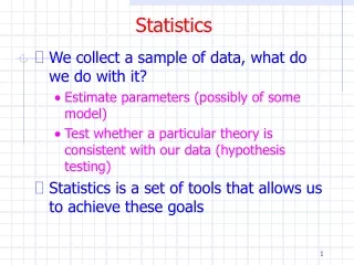
Statistics • We collect a sample of data, what do we do with it? • Estimate parameters (possibly of some model) • Test whether a particular theory is consistent with our data (hypothesis testing) • Statistics is a set of tools that allows us to achieve these goals
Statistics • Preliminaries
Statistics • Some common estimators are for the mean and variance
c2 Distribution • A common situation is that you have a set of measurements xi and you know the true value of each xit • How good are our measurements? • Similarly you may be comparing a histogram of data with another that contains expectation values under some hypothesis • How well do the data agree with this hypothesis? • Or if parameters of a function were estimated using the method of least squares, a minimum value of c2 was obtained • How good was the fit?
c2 Distribution • Assuming • The measurements are independent of each other • The measurements come from a Gaussian distribution • One can use the “goodness-of-fit” statistic c2 to answer these questions • In the case of Poisson distributed numbers, si2=xti, this is called Pearson’s c2 statistic
c2 Distribution • Chi-square distribution
c2 Distribution • The integrals (or cumulative distributions) between arbitrary points for both the Gaussian and c2 distributions cannot be evaluated analytically and must be looked up • What is the probability of getting a c2 > 10 with 4 degrees of freedom? • This number tells you the probability that random fluctuations (chance fluctuations) in the data would give a value of c2 > 10
c2 Distribution • Note the p-value is defined as • We’ll come back to p-values in a moment
c2 Distribution • 1- cumulative c2distribution
c2 Distribution • Often one uses the reduced c2 = c2/n
Hypothesis Testing • Hypothesis tests provide a rule for accepting or rejecting hypotheses depending on the outcome of a measurement
Hypothesis Testing • Normally we define regions in x-space that define where the data is compatible with H or not
Hypothesis Testing • Let’s say there is just one hypothesis H • We can define some test statistic t whose value in some way reflects the level of agreement between the data and they hypothesis • We can quantify the goodness-of-fit by specifying a p-value given an observed tobs in the experiment • Assumes t is defined such that large values correspond to poor agreement with the hypothesis • g is the pdf for t
Hypothesis Testing • Notes • p is not the significance level of the test • p is not the confidence level of a confidence interval • p is not the probability that H is true • That’s Bayesian speak • p is the probability, under the assumption of H, of obtaining data (x or t(x)) having equal or lesser compatibility with H as xobs
Hypothesis Testing • Flip coins • Hypothesis H is coin is fair (random) so ph=pt=0.5 • We could take t=|nh-N/2| • Toss coin N=20 times and observe nh=17 • Is H false? • Don’t know • We can say that probability of observing 17 or more heads assuming H is 0.0026 • p is the probability of observing this result “by chance”
Kolmogorov-Smirnov (K-S) Test • The K-S test is an alternative to the c2test when the data sample is small • It is also more powerful than the c2test since it does not rely on bins – though one commonly uses it that way • A common use is to quantify how well data and Monte Carlo distributions agree • It also does not depend on the underlying cumulative distribution function being tested
K-S Test • Data – Monte Carlo comparison
K-S Test • The K-S test is based on the empirical distribution function (ECDF) Fn(x) • For n ordered data points yi • This is a step function that increases by 1/N at the value of each ordered data point
K-S Test • The K-S statistic is given by • If D > some critical value obtained from tables, the hypothesis (data and theory distributions agree) is rejected
Statistics • Suppose N independent measurements xi are drawn from a pdf f(x;q) • We want want to estimate the parameters q • The most important method for doing this is the method of maximum likelihood • A related method in the case of least squares
Hypothesis Testing • Example • Properties of some selected events • Hypothesis H is these are top quark events • Working in x-space is hard so usually one constructs a test statistic t instead whose value reflects the compatibility between the data vector x and H • Low t – data more compatible with H • High t – data less compatible with H • Since f(x,H) is known, g(t,H) can be determined
Hypothesis Testing • Notes • p is not the significance level of the test • p is not the confidence level of a confidence interval • p is not the probability that H is true • That’s Bayesian speak • p is the probability, under the assumption of H, of obtaining data (x or t(x)) having equal or lesser compatibility with H as xobs • Since p is a function of r.v. x, p itself is a r.v • If H is true, p is uniform in [0,1] • If H is not true, p is peaked closer to 0
Hypothesis Testing • Suppose we observe nobs=ns+nb events • ns, nb are Poisson r.v.’s with means ns,nb • nobs=ns+nb is Poisson r.v. with mean n=ns+nb
Hypothesis Testing • Suppose nb=0.5 and we observe nobs=5 • Publish/NY Times headline or not? • Often we take H to be the null hypothesis – assume it’s random fluctuation of background • Assume ns=0 • This is the probability of observing 5 or more resulting from chance fluctuations of the background
Hypothesis Testing • Another problem, instead of counting events say we measure some variable x • Publish/NY Times headline or not?
Hypothesis Testing • Again take H to be the null hypothesis – assume it’s random fluctuation of background • Assume ns=0 • Again p is the probability of observing 11 or more events resulting from chance fluctuations of the background • How did we know where to look / how to bin? • Is the observed width consistent with the resolution in x? • Would a slightly different analysis still show a peak? • What about the fact that the bins on either side of the peak are low?
Least Squares • Another approach is to compare a histogram with a hypothesis that provides expectation values • In this case we’d compare a vector of Poisson distributed numbers (the histogram) with their expectation values ni=E[ni] • This is called Pearson’s statistic • If the ni are not too small (e.g. ni > 5) then the observed c2 will follow the chi-square pdf for N dof • Or more generally for N – number of fitted parameters • Same will hold true for N independent measurements yi that are Gaussian distributed
Least Squares • We can calculate the p-value as • In our example
Least Squares • In our example though we have many bins with a small number of counts or 0 • We can still use Pearson’s test but we need to determine the pdf f(c2) by Monte Carlo • Generate ni from Poisson, mean niin each bin • Compute c2 and record in a histogram • Repeat for a large number of times (see next slide)
Least Squares • Using the modified pdf would give p=0.11 rather than p=0.073 • In either case, we won’t publish
K-S Test • Usage in ROOT • TFile * data • TFile * MC • TH1F * jet_pt = data → Get(“h_jet_pt”) • TH1F * MCjet_pt = MC → Get(“h_jet_pt”) • Double_t KS=MCjet_pt→KolmogorovTest(jet_pt) • Notes • The returned value is the probability of the test • << 1 means the two histograms are not compatable • The returned value is not the maximum KS distance though you can return this with option “M” • Also available in statistical toolbox in MatLab
Limiting Cases Binomial Poisson Gaussian
Nobel Prize or IgNobel Prize? • CDF result
Kaplan-Meier Curve • A patient is treated for a disease. What is the probability of an individual surviving or remaining disease-free? • Usually patients will be followed for various lengths of time after treatment • Some will survive or remain disease-free while others will not. Some will leave the study. • A nonparametric method can be found using • Kaplan-Meier curve • Life table • Survival curve 36
Kaplan-Meier Curve • Calculate a conditional probability • S(tN) = P(t1) x P(t2) x P(t3) x … P(tN) • The survival function S(t) is equivalent to the empirical distribution function F(t) • We can write this as 37
Kaplan-Meier Curve • The square root of the variance of S(t) can be calculated as • Assuming the pk follow a Gaussian (normal) distribution, then the 95% CL will be 39
Gaussian Distribution • Some useful properties of the Gaussian distribution are • P(x in range m±s) = 0.683 • P(x in range m±2s) = 0.9555 • P(x in range m±3s) = 0.9973 • P(x outside range m±3s) = 0.0027 • P(x outside range m±5s) = 5.7x10⁻⁷ • P(x in range m±0.6745s) = 0.5
Confidence Intervals • Suppose you have a bag of black and white marbles and wish to determine the fraction f that are white. How confident are you of the initial composition? How does your confidence change after extracting n black balls? • Suppose you are tested for a disease. The test is 100% accurate if you have the disease. The test gives 0.2% false positive if you do not. The test comes back positive. What is the probability that you have the disease?
Confidence Intervals • Suppose you are searching for the Higgs and have a well-known expected background of 3 events. What 90% confidence limit can you set on the Higgs cross section • if you observe 0 events? • if you observe 3 events? • if you observe 10 events? • The ability to set confidence limits (or claim discovery) is an important part of frontier physics • How to do this the “correct” way is somewhat/very controversial
Confidence Intervals • Questions • What is the mass of the top quark? • What is the mass of the tau neutrino • What is the mass of the Higgs • Answers • Mt = 172.5 ± 2.3 GeV • Mv < 18.2 MeV • MH > 114.3 GeV • More correct answers • Mt = 172.5 ± 2.3 GeV with CL = 0.683 • 0 < Mv < 18.2 MeV with CL = 0.95 • Infinity > MH > 114.3 GeV with CL = 0.95
Confidence Interval • A confidence interval reflects the statistical precision of the experiment and quantifies the reliabiltiy of a measurement • For a sufficiently large data sample, the mean and standard deviation of the mean provide a good provide a good interval • What if the pdf isn’t Gaussian? • What if there are physical boundaries? • What if the data sample is small? • Here we run into problems
Confidence Interval • A dog has a 50% probability of being 100m from its master • You observe the dog, what can you say about its master? • With 50% probability, the master is within 100m of the dog • But this assumes • The master can be anywhere around the dog • The dog has no preferred direction of travel
Confidence Intervals • Neyman’s construction • Consider a pdf f(x;θ) = P(x|θ) • For each value of θ, we construct a horizontal line segment [x1,x2] such that P(x Î[x1,x2]|θ) = 1-a • The union of such intervals for all values of θ is called the confidence belt
Confidence Intervals • Neyman’s construction • After performing an experiment to measure x, a vertical line is drawn through the experimentally measured value x0 • The confidence interval for θis the set of all values of θfor which the corresponding line segment [x1,x2] is intercepted by the vertical line