Machine Learning: Basic Introduction

1. Machine Learning: Basic Introduction Jan Odijk January 2011 LOT Winter School 2011

2. Overview • Introduction • Rule-based Approaches • Machine Learning Approaches • Statistical Approach • Memory Based Learning • Methodology • Evaluation • Machine Learning & CLARIN

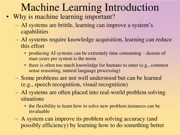
3. Introduction • As a scientific discipline • Studies algorithms that allow computers to evolve behaviors based on empirical data • Learning: empirical data are used to improve performance on some tasks • Core concept: Generalize from observed data

4. Introduction • Plural Formation • Observed: list of (singular form, plural form) • Generalize: predict plural form given a singular form for new words (not in observed list) • PoS tagging • Observed: text corpus with PoS-tag annotations • Generalize: predict Pos-Tag of each token from a new text corpus

5. Introduction • Supervised Learning • Map input into desired output, e.g. classes • Requires a training set • Unsupervised Learning • Model a set of inputs (e.g. into clusters) • No training set required

6. Introduction • Many approaches • Decision Tree Learning • Artificial Neural Networks • Genetic programming • Support Vector Machines • Statistical Approaches • Memory Based Learning

7. Introduction • Focus here • Supervised learning • Statistical Approaches • Memory-based learning

8. Rule-Based Approaches • Rule based systems for language • Lexicon • Lists all idiosyncratic properties of lexical items • Unpredictable properties e.g man is a noun • Exceptions to rules, e.g. past tense(go) = went • Hand-crafted • In a fully formalized manner

9. Rule-Based Approaches • Rule based systems for language (cont.) • Rules • Specifies regular properties of language • E.g. direct object directly follows verb (in English) • Hand-crafted • In a fully formalized manner

10. Rule-Based Approaches • Problems for rule based systems • Lexicon • Very difficult to specify and create • Always incomplete • Existing dictionaries • Were developed for use by humans • Do not specify enough properties • Do not specify the properties in a formalized manner

11. Rule-Based Approaches • Problems for rule based systems (cont.) • Rules • Extremely difficult to describe a language (or even a significant subset of language) by rules • Rule systems become very large and difficult to maintain • (No robustness (‘fail softly’) for unexpected input)

12. Machine Learning • Machine Learning • A machine learns • Lexicon • Regularities of language • From a large corpus of observed data

13. Statistical Approach • Statistical approach • Goal: get output O given some input I • Given a word in English, get its translation in Spanish • Given acoustic signal with speech, get the written transcription of the spoken word • Given preceding tags and following ambitag, get tag of the current word • Work with probabilities P(O|I)

14. Statistical Approach • P(A) probability of A • A an event (usually modeled by a set) • Event space=all possible event elements: Ω • 0 ≤ P(A) ≤ 1 • For finite event space, and a uniform distribution: P(A) = |A| / |Ω|

15. Statistical Approach • Simple Example • A fair coin is tossed 3 times • What is the probability of (exactly) two heads? • 2 possibilities for each toss: Heads or Tails • Solution: • Ω = {HHH, HHT, HTH, HTT, THH, THT, TTH, TTT} • A = {HHT, HTH, THH} • P(A) = |A| / |Ω| = 3/8

16. Statistical Approach • Conditional Probability • P(A|B) • Probability of event A given that event B has occurred • P(A|B) = P (A ∩ B) / P(B) (for P(B)>0) A A∩B B

17. Statistical Approach • A fair coin is tossed 3 times • What is the probability of (exactly) two heads (A) if the first toss has occurred and is H (B)? • Ω = {HHH, HHT, HTH, HTT, THH, THT, TTH, TTT} • A = {HHT, HTH, THH} • B = {HHH,HHT,HTH,HTT} • A ∩ B = {HHT, HTH} • P(A|B)=P(A∩B) / P(B) = 2/8 / 4/8 = 2 / 4 = ½

18. Statistical Approach • Given • P(A|B)=P(A∩B) / P(B)  (multiply by P(B)) • P(A∩B) = P(A|B) P(B) • P(B∩A) = P(B|A) P(A) • P(A∩B) = P(B∩A)  • P(A∩B) = P(B|A) P(A) • Bayes Theorem: • P(A|B) = P(A∩B)/P(B) = P(B|A)P(A) / P(B)

19. Statistical Approach • Bayes Theorem Check • Ω = {HHH, HHT, HTH, HTT, THH, THT, TTH, TTT} • A = {HHT, HTH, THH} • B = {HHH,HHT,HTH,HTT} • A ∩ B = {HHT, HTH} • P(B|A) = P(B∩A) / P(A) = 2/8 / 3/8 = 2/3 • P(A|B) = P(B|A)P(A) / P(B) = (2/3 * 3/8) / (4/8) = 2 * 6/24= 1/2

20. Statistical Approach • Statistical approach • Using Bayesian inference (noisy channel model) • get P(O|I) for all possible O, given I • take that O given input I for which P(O|I) is highest: Ô • Ô = argmaxO P(O|I)

21. Statistical Approach • Statistical approach • How to obtain P(O|I)? • Bayes Theorem • P(O|I) =

22. Statistical Approach • Did we gain anything? • Yes! • P(O) and P(I|O) often easier to estimate than P(O|I) • P(I) can be ignored: it is independent of O. • (though we have no probabilities anymore) • In particular: • argmaxO P(O|I) = argmaxO P(I|O) * P(O)

23. Statistical Approach • P(O) (also called the Prior probability) • Used for the language model in MT and ASR • cannot be computed: must be estimated • P(w) estimated using the relative frequency of w in a (representative) corpus • count how often w occurs in the corpus • Divide by total number of word tokens in corpus • = relative frequency ; set this as P(w) • (ignoring smoothing)

24. Statistical Approach • P(I|O) (also called the likelihood) • Cannot easily be computed • But estimated on the basis of a corpus • Speech recognition: • Transcribed speech corpus •  Acoustic Model • Machine translation • Aligned parallel corpus •  Translation Model

25. Statistical Approach • How to deal with sentences instead of words? • Sentence = w1..wn • P(S) = P(w1)*..*P(wn)? • NO: This misses the connections between the words • P(S) = (chain rule) • P(w1)P(w2|w1)P(w3|w1w2)..P(wn|w1..wn-1)

26. Statistical Approach • N-grams needed (not really feasible) • Probabilities of n-grams are estimated by the relative frequency of n-grams in a corpus • Frequencies get too low for n-grams n>=3 to be useful • In practice: use bigrams, trigrams (4-grams) • E.g. Bigram model: • P(S) = P(w1w2)* P(w2w3)..* P(wn-1wn)

27. Memory Based Learning • Classification • Determine input features • Determine output classes • Store observed examples • Use similarity metrics to classify unseen cases

28. Memory Based Learning • Example: PP-attachment • Given a input sequence V ..N.. PP • PP attaches to V?, or • PP attaches to N? • Examples • John ate crisps with Mary • John ate pizza with fresh anchovies • John had pizza with his best friends

29. Memory Based Learning • Input features (feature vector): • Verb • Head noun of complement NP • Preposition • Head noun of complement NP in PP • Output classes (indicated by class labels) • Verb (i.e. attaches to the verb) • Noun (i.e. attaches to the noun)

30. Memory Based Learning • Training Corpus:

31. Memory Based Learning • MBL: Store training corpus (feature vectors + associated class in memory) • for new cases • Stored in memory? • Yes: assign associated class • No: use similarity metrics

32. Similarity Metrics • (actually : distance metrics) • Input: eats pizza with Liam • Compare input feature vector X with each vector Y in memory: Δ(X,Y) • Comparing vectors: sum the differences for the n individual features Δ(X,Y) = Σni=1δ(xi,yi)

33. Similarity Metrics • δ(f1,f2) = • (f1,f2 numeric): • (f1-f2)/(max-min) • 12 – 2 = 10 in a range of 0 .. 100  10/100=0.1 • 12 - 2 = 10 in a range of 0 .. 20  10/20 = 0.5 • (f1,f2 not numeric): • 0 if f1= f2 no difference  distance = 0 • 1 if f1≠ f2 difference  distance = 1

34. Similarity Metrics

35. Similarity Metrics • Look at the “k nearest neighbours” (k-NN) • (k = 1): look at the ‘nearest’ set of vectors • The set of feature vectors with ids {2,3,4} has the smallest distance (viz. 2) • Take the most frequent class occurring in this set: Verb • Assign this as class to the new example

36. Similarity Metrics • with Δ(X,Y) = Σni=1δ(xi,yi) • every feature is ‘equally important; • Perhaps some features are more ‘important’ • Adaptation: • Δ(X,Y) = Σni=1 wi * δ(xi,yi) • Where wi is the weight of feature i

37. Similarity Metrics • How to obtain the weight of a feature? • Can be based on knowledge • Can be computed from the training corpus • In various ways: • Information Gain • Gain Ratio • χ2

38. Methodology • Split corpus into • Training corpus • Test Corpus • Essential to keep test corpus separate • (Ideally) Keep Test Corpus unseen • Sometimes • Development set • To do tests while developing

39. Methodology • Split • Training 50% • Test 50% • Pro • Large test set • Con • Small training set

40. Methodology • Split • Training 90% • Test 10% • Pro • Large training set • Con • Small test set

41. Methodology • 10-fold cross-validation • Split corpus in 10 equal subsets • Train on 9; Test on 1 (in all 10 combinations) • Pro: • Large training sets • Still independent test sets • Con : training set still not maximal • requires a lot of computation

42. Methodology • Leave One Out • Use all examples in training set except 1 • Test on 1 example (in all combinations) • Pro: • Maximal training sets • Still independent test sets • Con : requires a lot of computation

43. Evaluation

44. Evaluation • TP= examples that have class C and are predicted to have class C • FP = examples that have class ~C but are predicted to have class C • FN= examples that have class C but are predicted to have class ~C • TN= examples that have class ~C and are predicted to have class ~C

45. Evaluation • Precision = TP / (TP+FP) • Recall = True Positive Rate = TP / P • False Positive Rate = FP / N • F-Score = (2*Prec*Rec) / (Prec+Rec) • Accuracy = (TP+TN)/(TP+TN+FP+FN)

46. Example Applications • Morphology for Dutch • Segmentation into stems and affixes • Abnormaliteiten -> abnormaal + iteit + en • Map to morphological features (eg inflectional) • liepen-> lopen + past plural • Instance for each character • Features: Focus char; 5 preceding and 5 following letters + class

47. Example Applications • Morphology for Dutch Results Prec Rec F-Score • Full: 81.1 80.7 80.9 • Typed Seg: 90.3 89.9 90.1 • Untyped Seg: 90.4 90.0 90.2 • Seg=correctly segmented • Typed= assigned correct type • Full = typed segm + correct spelling changes

48. Example Applications • Part-of-Speech Tagging • Assignment of tags to words in context • [word] -> [(word, tag)] • [book that flight] -> • [(book, verb) (that,Det) (flight, noun)] • Book in isolation is ambiguous between noun and verb: marked by an ambitag: noun/verb

49. Example Applications • Part-of-Speech Tagging Features • Context: • preceding tag + following ambitag • Word: • Actual word form for 1000 most frequent words • some features of the word • ambitag of the word • +/-capitalized • +/-with digits • +/-hyphen

50. Example Applications • Part-of-Speech Tagging Results • WSJ: 96.4% accuracy • LOB Corpus: 97.0% accuracy