Download
1 / 167
1.68k likes | 1.9k Views
CP Violation and all that. Brian Meadows University of Cincinnati. Lecture I Outline. CP Violation and how it can come about. The CKM model for CPV Unitarity triangles B factory measurements Other triangles Mixing and CPV Present experimental situation Summary and Discussion.

E N D
CP Violation and all that. Brian Meadows University of Cincinnati Brian Meadows, U. Cincinnati.
Lecture I Outline • CP Violation and how it can come about. • The CKMmodel for CPV • Unitarity triangles • B factory measurements • Other triangles • Mixing and CPV • Present experimental situation • Summary and Discussion Brian Meadows, U. Cincinnati
CP Violation (CPV ) - very brief History • CPV is observable as a particle/antiparticle asymmetry in the rates of transitions: for processeswith initial state i and final state f • CPV was discovered (Fitch and Cronin 1963) in decays to p+p- states (with CP=+1) by long-lived KL mesons that were formerly found to decay only to (with CP=-1). • It was next seen as an asymmetry in decays (Bars indicate antiparticle conjugate states)
CPV – very brief History (2) • Theoretically, there was much speculation on the source of CPV – whether from mixing or decay (“direct”). • In 1973, Kobayashi and Moskawa suggested the current 3-family nature of the SM and pointed out that it led to the possibility for CPV. • Experimentally, CPV was not observed anywhere other than in neutral K decays for ~40 years when, much as predicted by KM, the BaBar and Belle experiments observed its interference with mixing in decays of B0mesons toJ/Ã Ksfinal states (CP=-1). • First evidence for direct CPV in B decays was later observed in 2004 by the BaBar and Belle experiments. Brian Meadows, U. Cincinnati
CPV and Baryogenesis • CPV is also needed to account for excess of baryons over anti-baryons in our universe. • This excess is only a small fraction of the observed number of photons . • Sakharov (1967) held that this requires: • Baryon number violating processes - • CPV so that, for any baryon-violating process, • A period in the history of the universe when it was not in thermal equilibrium. In thermal equilibrium (T invariance), CPT invariance is equivalent to CP invariance! • CPT violation alone, could also generate • This would also violate locality, causality and Lorentz invariance.
B = r B1+ (1 - r) B2 B = r (-B1 ) + (1 – r )(-B2 ) Early Universe – an Illustration • Consider a particle which has just two decay modes to final states f1,2 with baryon numbers B1,2 (not necessarily the same) and branching fractions r and (1 – r ). • CPT invariance requires anti-particle to have the same total decay ratesbut CP violation can allow r to differ from r. • Decay of each pair (initially B = 0): results in a change in number of baryons ¢B =(r – r ) (B1 - B2 ) • Baryon-dominant universe requires this be positive, so: • - baryon number is violatedfor at least one decay mode AND • - there isCPV
CPV and Field Theory • The SM Lagrangian is Hermitian and includes terms like where the are scalar operators defined from quark and lepton fields and the aiare couplings. • CP -invariance requires that all couplings can be made real with a suitable choice of phases for the fields. • In the SM, charged EW terms are of the form These all involve the CKM matrixVCKM that has a phase that depends on specific flavor couplings The effects of such a phase cannot be removed, for all flavors, simply by re-phasing the quark fields CPV
More about the CKM Matrix • This is a 3x3 unitary transformation • Defined by rotations about 3 axes by angles q12, q13, q23 where sij= sin qij and cij= sin qij, and (important) a phase • Then Brian Meadows, U. Cincinnati
Wolfenstein Expansion • So • The terms have a numerical hierarchy that suggests an expansion in powers of the Cabibbo angle = Vus : where A, and are parameters of order one. VCKM Brian Meadows, U. Cincinnati
Arg{Vub} = - d s b u c t (, ) Vtb*Vtd Vcb*Vcd Vub*Vud Vcb*Vcd Arg{Vtd} = -b (1, 0) (0, 0) Get to know the CKM • Magnitudes: Memorize the power of for each term. • Phases: Remember the phases for the two terms circled • Labels for rows/columns VCKM “The” unitarity triangle
Vtsacquires a phase at order 4 Other Expansions • This expansion preserves unitarity below order 4. • Preserving unitarity to all orders is possible (Buras, Lautenbacher and Ostermaier, 1994) with parameters: • At order 5, this leads to Phase(°) of Vub is unchanged Vcdacquires a phase at order 5 Brian Meadows, U. Cincinnati
Unitarity Triangles d s b (K system) d•s* = 0 u c t (Bs system) s•b* = 0 (Bd system) d•b* = 0 apply unitarity constraint to pairs of columns from P. Burchat Florida State U: Tallahasee, FLA, April 21 2003. Brian Meadows, U. Cincinnati
(Three more) Unitarity Triangles d s b (D system) u•c* = 0 u c t (“T” system) c•t* = 0 (“T’” system) u•t* = 0 All six triangles have the same area. A nonzero area is a measure of CP violation and is an invariant of the CKM matrix. Apply unitarity constraint to pairs of rows from P. Burchat Florida State U: Tallahasee, FLA, April 21 2003. Brian Meadows, U. Cincinnati
Vtb*Vtd Vub*Vud Vcb*Vcd “The (Usual) Unitarity Triangle” d s b [Technically, this is the “bd” triangleAlso called the “Bd” triangle]. u c t Orientation of triangle has no physical significance. Only relative angle between sides is significant. Apply unitarity constraint to these two columns from P. Burchat Florida State U: Tallahasee, FLA, April 21 2003. Brian Meadows, U. Cincinnati
The Usual Unitarity Triangle (, ) Vtb*Vtd Vcb*Vcd Vub*Vud Vcb*Vcd (1, 0) (0, 0) d s b u c t Apply unitarity constraint to these two columns from P. Burchat Florida State U: Tallahasee, FLA, April 21 2003. Brian Meadows, U. Cincinnati
The bd Unitarity Triangle before B Factories CKM parameters and obtained from the observables K, xd=Md/G, |Vub|,|Vcb| a g b From P. Burchat and J. Richman, Rev. Mod. Phys., 67 (1995) 893-976
The bd Unitarity Triangle Today CKM parameters can be used to predict other observables K, Md, Ms, BF(B), Vub, sin2, , Vcb, lattice, … CKMFitter UTFit
CKM Predictions Fits to measured values give values for CKM parameters: Some “tension” exists and it will be important to continue to check the CKM paradigm with more precise measurements. • Significant discrepancies exist: • sin2 ~3 low • BF(B) 2.7 high • Is CKM model in question? arXiv:1104.2117 [hep-ph]
Measurements of CKM elements |Vud|0.974250 0.0022Super-allowed decay. Best measurement |Vus|0.2253 0.0008Kl2 & Kl3 (need lattice) and K. |Vub|0.00392 0.00046BXl, Bu decays. Some discrepancies |Vcd|0.230 0.011Charm prod by ’s. DKl needs theory |Vcs|1.04 0.06 DKl , Dsl (theory limited) |Vcb|0.0409 0.0007BDl , BD*l , lattice |Vtd|0.0081 0.0005 Bd Mixing, lattice prediction for |Vts|/|Vtd| |Vts|0.0387 0.0023Bs Mixing |Vts|0.88 0.07Single top production (CDF,D0,Atlas,CMS)
Measuring , and from B Decays • Anatomy of Weak Decays – weak and strong phases • Mixing in the neutral B meson system • Three types of CPV • Mixing-induced CPV • Ways to measure weak phase
s Anatomy of Weak Decays u c s u u Tree (T) h + u s u h - s K+ h + h - K - • Weak (short range)|W|ei • Neither I, U, V-spin, P nor CP • are (necessarily) conserved. 3 stages K+ D0 K - Hadronisation • Strong (long range)|S|eid • Everything conserved. • I -spin, P, CP, .. Scattering [Small E/M component may not conserve I ]
Space-time regimes (2) The two space-time ranges differ greatly so that we can write overall decay amplitude as a product UnderCPweak phase flips sign but does not so This can give rise to CPV Similar considerations govern the behavior of all processes involving weak interactions. Strong phase Weak phase
Hadron – Friend or Foe! • Final states often consist of multiple, strongly interacting hadrons. At one time, such systems were thought to obscure the “more fundamental” aspects of the short-range weak interactions which lay at the heart of CPV. • It was later realized that the relative phases of the hadronic interaction processes can be measured from the density of decays in phase space (e.g. position in a Dalitz plot). • The phases so measured consist of a strong and a weak component as just discussed, and so actually provide invaluable information on the short range weak phases in the amplitudes governing the decay. • Another “useful nuisance” is the phenomenon of mixing that we discuss next ….
Dalitz plot for D0KS+- Weak phases through the Hadron eye • Dalitz plot for D0KS+- • The flavour of the KS (ie K0+-) is undefined, so both K*0 and K*0 can be produced at the quark level: • K*0 (csud cos c2 ) • K*0 (cdsu -sin c2 ) • NOTE change of sign of weak (ie ”production” amplitude) • Observe the K*0 (horizontal band) !
Neutral Meson (M0) Systems • Flavour eigenstates are not mass eigenstates so they mix: • We define four mixing parameters as • The flavour states oscillate in time differently • Unless p = q, these are in not phase and “mixing-induced”, time-dependent CPV asymmetry occurs.
Mixing and CPV • Mixing is an ubiquitous phenomenon readily observed in the K0, D0, B0 and Bs neutral meson systems . • The T0 could mix, but will decay before mixing can occur. • 0, 0, ’ mesons do not mix since they are their own anti-particles. • The D0 system is the only up-type meson that mixes. The SM greatly suppresses this, however. • Mixing can lead to CPV and, in bringing meson and anti-meson decays into interference, it can allow the measurement of the weak decay phases involved.
u, c, t W d d b b + W W u, c, t d d W b b u, c, t u, c, t Where does mixing come from ? • Transitions that change flavour (S, C or B=2) are possible via box diagrams, illustrated for Bd0 below: • A weak phase in q/p, M=Arg{q/p}, leads to CPV in mixing. for B0 system for K0 system We return to D0system later for Bs system
Observation of Mixing • For mixing to be observed, M0 (or M0) must be flavour- tagged at time t=0 and then again when it decays • Decays to final states accessible to both M0 and M0 are possible, especially when the final state is comprised of hadrons. • Rates for initial M0 and initial M0 are decays are not equal if q is not equal to p (CPV in mixing). • In such cases, interference between M0 and M0 decays occurs and can be used to measure mixing and CPV parameters.
(M0f) Mixing brings decays from M and M into interference M 0 “f” (M 0f) Mix (M 0 M 0) Decays to states accessible to both M0 and M0 • For such decays we define amplitudes • The important parameter is and its measurement is crucial to CPV studies. Opens the possibility to measure the weak phase The phase of f includes M and the weak and strong phases in the decay.
Time-dependent “Dalitz plot fits” • The effects of mixing can be included in a fit to a multi-body hadronic final state f arising from decays of neutral mesons, such as M0. • The t-dependent decay amplitude for a state M0 at t =0 is: where and are linear combinations of amplitudes (eg “isobar”, etc.) normally present in a fit at t =0. They depend upon the position in the phase space • This can be written in the form: • The phase space and time t dependencesfactorize.
Time-dependent “Dalitz plot fits” • The Dalitz plot density is then • The Dalitz plot density can be written, similarly, for M0. • It is not, in general, the same as that for the M0. • Note that • mixing brings bothM0 andM0 into interference in the decay ofM0; • The phase space time t dependences factorize. • The parameter becomes It is important to point out that the weak phase, W, of f is assumed not to depend on
Three types of CPV • In the mixing (“indirect CPV”) • In the decay (“direct CPV”) • In interference between mixing and decay (“indirect CPV” – a.k.a. “mixing-induced CPV”)
Direct CPV When two (or more) amplitudes,TandP for example, mediate the decay process, then decay amplitudes are This leads to a CP asymmetry in decay rates NOTE ACP = 0unless ACP is largest when P=T. Wm and Mary, VA, June 11, 2012. Brian Meadows, U. Cincinnati
Mixing-induced CPV in M0 Decays Using the two different time-dependent flavour states, we derive decay rates ( ) for M0(M0) to f that also differ: and result in a time-dependentCP asymmetry (TDCPV)
Decay (weak) Decay (strong) BUT only if we know the strong phasef. Mixing (weak) Time-dependent CPV analysis • The parameter f encodes the weak and strong phases into this asymmetry So measuring thisM0-M0asymmetry as a function of time allows measurement of the weak phaseW = M - 2f
Time-dependent CPV analysis • Three possibilities for measuring f in a TDCPV analysis: 1. If f is a CP eigenstate fCP (e.g. +-, Ks, J/ KL, etc.). strong phase of same as that of so 2. Similarly, if f is CP self conjugate (sum of CP-even and CP-odd states) e.g. 0Ks, J/ K*, etc. strong phases of linked to those of so 3. If f is a multi-hadron system - Amplitude analysis of hadrons allows measurement off From Dalitz Plot, etc.
(Belle chose to use “A”=-C ) Application to B0 Decays at BaBar/Belle • For B0 mesons, y 0 so their decay rates are: with time-dependent (TD)CP asymmetry where • CPV analyses at the B factories focus on measuring C (direct CPV) and S (to extract the weak phase of f). C=0 in absence of direct CPV S measurable Only in TDCPV
Original B Factory goals • Use Y(4S) decays to B0-B0 pairs – one is “flavour tagged” as either B0 or B0 and other B0 decays in a CP eigenstate. • Measure t between the two decays and the CP asymmetry at each t. • Figure shows ideal case for J/Ks • no experimental effects. • Asymmetry is large.
b c d d W c b s s c d d c Sin 2: B0J/Ks (bccs) B mix phase: Penguin phase P is the SAME! Tree phase: Ks mix phase: Comes with K0 Vtb 1 ; Arg{Vtd} = - ; Arg{VcbVcd*} 0 Weak phase:
u d Sin 2a: B0+- (buud) d b d W u b u u d d d B mix phase: Penguin phase P is NOT the same! Tree phase: Needs to be measured VtbVud1 ; Arg{Vtd} = - ; Arg{Vub}= Weak phase:
b u s s W u b d d d, u s s d, u Sin 2g: BsKs (buud) Bs mix phase: Experimentally impossible at B factories, though! Penguin phase P is NOT the same! Tree phase: Ks mix phase: Comes with K0 VtbVud1; Arg{VtsVcs*} 0 ; Arg{Vub} ; Arg{Vcd} 0 Weak phase:
Actual Achievements of the B factories have far exceeded these goals • Many other modes were used, including: • those where penguin contributions were important or even dominant • some requiring the invocation of SU(2) symmetry (I, U and V-spin) • non CP-eigenstates • multi-hadron hadron systems requiring TD Dalitz plot amplitude analyses. • various vector-vector modes (separating out the longitudinal helicity components (CP=+1) • A credible set of methods to determine that did not involve TD studies of Bs mesons were also developed.
What might we expect from the future ? • Yet more modes (LHCb and SuperB/Belle2) • Multi-hadron modes with 4-body (or higher dimension) amplitude analyses separating out the CP-odd or CP-even helicity components (LHCb and SuperB/Belle2) • Full use of more precise strong phase measurements from charm threshold data (BES3 and SuperB) • TD studies of Bs mesons (LHCb). • Much information on direct or time-integrated CPV(mostly BES3/Panda but also LHCb/SuperB/Belle2). • CPV studies of the charm triangle and further understanding of the origin for LHCb evidence of direct CPV in D0+- and D0K+K- decays (LHCb and SuperB/Belle2).
The B Factory Experiments Asymmetric 4 Detectors KEK-b at KEK 8 Gev e- on 3.5 GeV e+ PEP-II as SLAC 9 Gev e- on 3.1 GeV e+
p+ B0 / B0 e+ e- — B0 / B0 e ±, m ±, K± tag Dz =c t Dz ~ 255 mm for PEP-II: 9.0 GeV on 3.1 GeV ~ 200 mm for KEKB: 8.0 GeV on 3.5 GeV The Asymmetric-Energy B Factories (4S) Florida State U: Tallahasee, FLA, April 21 2003. Brian Meadows, U. Cincinnati
Original B Factory plan • Use Y(4S) decays to B0-B0 pairs – one is “flavour tagged” as either B0 or B0 and other one decays in a CP eigenstate. • Decay rates and CP asymmetry shown for B0J/ Ks (CP eigenstate decay) mode. • Ideal case shown, no experimental effects included. • Asymmetry is large, but experimental effects reduce it considerably.
Backgrounds in B meson samples • Typical variables used Particle ID also of vital importance