Download
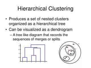
1 / 29
290 likes | 556 Views
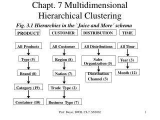
PRODUCT. CUSTOMER. DISTRIBUTION. TIME. All Products. All Customer. All Distributions. All Time. Type (5). Sales. Region (8). Year (3). Organization (5). Month (12). Brand (8). Distribution. Nation (7). Channel (3). Category (19). Trade. Type (2). Container (10). Business.

E N D
PRODUCT CUSTOMER DISTRIBUTION TIME All Products All Customer All Distributions All Time Type (5) Sales Region (8) Year (3) Organization (5) Month (12) Brand (8) Distribution Nation (7) Channel (3) Category (19) Trade Type (2) Container (10) Business Type (7) Chapt. 7 Multidimensional Hierarchical Clustering Fig. 3.1 Hierarchies in the `Juice and More´ schema Prof. Bayer, DWH, Ch.7, SS2002
PRODUCT DISTRIBUTION 2180 rows 12 rows PRODKEY DISTKEY TYPE SALESORG BRAND CHANNEL FACT 26M rows CATEGORY ... PRODKEY CONTAINER CUSTKEY ... DISTKEY TIMEKEY CUSTOMER 7064 rows SALES CUSTKEY DISTCOST REGION TIME ... 36 rows NATION TIMEKEY TRADE-TYPE YEAR BUSINESS-TYPE MONTH ... (b) Prof. Bayer, DWH, Ch.7, SS2002
Size of completely aggregated Cube (6*9*20*11)*(9*8*3*8)*(6*4)*(4*13) ------------------------------------------------ = (5*8*19*10)*(8*7*2*7)*(5*3)*(3*12) 4*6*6*9*11*13 185.328 -------------------- = ----------- = 7.96 larger than base cube 5*5*7*7*19 23.275 Base Cube has 2.245.024.000 cells * 4 B ~ 9 GB Number of available facts: 26 million Prof. Bayer, DWH, Ch.7, SS2002
Sparsity: 26*106 -------------- = 0,0116 2,245* 109 100 - 1.16 = 98.84 % sparsity Prof. Bayer, DWH, Ch.7, SS2002
Hierarchically aggregated Cube (1+5+40+760+7600) = 8406 (1+8+56+112+784) = 961 (1+5+15) = 21 (1+3+24) = 28 P = 4.749.961.608 Size of base cube 2.145.024.000 Number of aggregate cells 2.504.937.608 ==> Juice and More database has 96times more hierarchically aggregated cells than occupied base cells! Prof. Bayer, DWH, Ch.7, SS2002
Select <MEASURE AGGREGATION> From Fact F, Customer C, DISTRIBUTION D, Product P, Time T Where F. ProdKey = P. ProdKey AND F. CustKey = C. CustKey AND F.TIMEKEY = T.TIMEKEY AND F.DISTKEY = D.DISTKEY AND <CUSTOMER RESTRICTION> AND <DISTRIBUTION RESTRICTION> AND <PRODUCT RESTRICTION> AND <TIME RESTRICTION> Star-Joins Restrictions on several dimension tables, which are then joined with fact table In addition: grouping, computation of aggregates, sorting of results. Example: Prof. Bayer, DWH, Ch.7, SS2002
Select <MEASURE AGGREGATION> From Fact F Where F. ProdKey BETWEEN Pkey1 AND Pkey2 AND F. DistKey BETWEEN Dkey1 AND Dkey2 AND F. CustKey BETWEEN Ckey1 AND Ckey2 AND F. TimeKey BETWEEN Tkey1 AND Tkey2 Prof. Bayer, DWH, Ch.7, SS2002
Key Question: • How to compute star-joins efficiently? • Secondary indexes on foreign keys of fact table (standard B-trees), see chapter 5 for details • - intersect result lists • retrieve tuples from fact table randomly • Bitmaps Prof. Bayer, DWH, Ch.7, SS2002
bitmap for organization 34 % of 1.....1.11 1.1...1.1. 1.1...1.1. ...1.1.... ..1.1...1. = „TM“ tuples bitmap for region 32 % of 11.1...... 1.11.....1 .1.1..1... 1.1.1..... .1..1.1... = „ Asia “ tuples result of bitmap intersection 10 % of 1......... 1.1....... ......1... .......... ....1..... tuples 80 % of accessed disk pages Page 1 Page 2 Page 3 Page 4 Page 5 pages (shaded) Bitmap Index Intersection Prof. Bayer, DWH, Ch.7, SS2002
Problem: for small result sets of a few %, almost all pages of the facts table must be fetched from disk, if the hits in the result set are not clustered on disk. Ex: with 8 KB pages 20 to 400 tuples per page, i.e. at 0.25% to 5% hits in the result almost all pages must be fetched. At least tuple clustering, preferably page clustering, are desirable, but how?? Goal: Code hierarchies in such a way, that for star-joins with the Fact table we have to join only with a query box on the Fact table Prof. Bayer, DWH, Ch.7, SS2002
0 = m {OJ 0.33L; OJ 0.7L; OJ 1L; Apple Juice 0.5L; 1L} 1 1 1 = = m {OJ 0.33L; OJ 0.7L; OJ 1L} m { Apple Juice 0.5L Apple Juice 1L} 1 2 2 2 2 2 2 = = = = = m {OJ 0.33L} m {OJ 0.7L} m { OJ 1L} m {A-Juice 0.5L} m {A-Juice 1L} 1 2 3 4 5 Level Label Legend: Member Label (e.g., 0.7L) Member Ordinal (e.g.,1) Basic Idea for Multidimensional Clustering All All Products AppleJuice Orange Juice Apple Juice Product Category 0 1 0 0,33L 1 0,7L 2 1L 0 0,5L 1 1L Example Hierarchy in Member Set Representation Prof. Bayer, DWH, Ch.7, SS2002
Dimension D consists of Value Set V = [[ v1, v2, ... vn ]] Hierarchy H of height h consisting of h+1 hierarchy levels H = [[L0 , L1,..., Lh ]] Level Liis a set of sets = [[m1i, ..., mji ]] with mki V mki get names, e.g. „Orange Juice“ as label(m11), in general label(mki) Constraint: every mli+1 must be a subset of some mki Prof. Bayer, DWH, Ch.7, SS2002
Hierarchic Relationships The children of mki are all those sets mli+1 of the lower level i+1 with the property: mli+1 mki , formally: children(mki ) := [[mli+1Li+1 : mli+1mki ]] parent(mki ) := [[mli-1Li-1 : mli-1mki ]] Principle: the children of m are numbered by the bijective function ordm starting at 1 or 0 Prof. Bayer, DWH, Ch.7, SS2002
Hierarchic Relationships The children of mki are all those sets mli+1 of the lower level i+1 with the property: mli+1 mki , formally: children(mki ) := [[mli+1Li+1 : mli+1mki ]] parent(mki ) := [[mli-1Li-1 : mli-1mki ]] Principle: the children of m are numbered by the bijective function ordm starting at 1 or 0 Prof. Bayer, DWH, Ch.7, SS2002
Enumeration and Surrogate Functions Let A be an enumeration type A = [[ a0, a1, ... ak ]] f : A --> (0, 1 ,..., k ) defined as f (ai ) = i then i is called the surrogate of ai Prof. Bayer, DWH, Ch.7, SS2002
Hierarchies and composite Surrogates Basic Idea: concatenate the surogates of successive hierarchy levels (compound surrogates cs) Note: the root ALL of the hierarchy is not encoded Def: compound surrogate cs for hierarchy H ordm : children (m) --> [[0, 1, ..., |children(m)| -1]] cs (H, mi) := ord father (mi) (mi) if i=1 :=cs (H, father ( mi)) ord father (mi) (mi) otherwise Prof. Bayer, DWH, Ch.7, SS2002
f(REGION) REGION South Europe 0 Middle Europe 1 Northern Europe 2 Western Europe 3 North America 4 Latin America 5 Asia 6 Australia 7 (a) Example: Prof. Bayer, DWH, Ch.7, SS2002
CUSTOMER South Europe North America Asia Australia 0 7 4 6 ... ... USA Canada Retail 0 1 Wholesale 0 1 Wholesale Retail Kana ´s Sushi Bar 0 1 ... ... Bar ... ... 2 Joe ‘sSportsBar ... ... Surrogates for Region and the entire Costumer Hierarchy Prof. Bayer, DWH, Ch.7, SS2002
Example: the path North America --> USA --> Retail --> Bar has the compound surrogate 4112 Next Idea: for every hierarchy level determine the higest branching degree (plus a safety margin for future extensions) and code by fixed number of bits. surrogates (H,i) := max [[ cardinality (children (H,m)) : m level (H, i-1) ]] Prof. Bayer, DWH, Ch.7, SS2002
let li := log2 surrogates (H,i) then li bits are needed for the surrogates of level i let be a path = m0 m1 m2 ... mh to a leaf mh of hierarchy H: Prof. Bayer, DWH, Ch.7, SS2002
cs (H,) = cs (H,mh) + := + ... + Prof. Bayer, DWH, Ch.7, SS2002
Example: cs (H, Bar) = 100 001 1 010 = 538 l1=3 l2=3 l3=1 l4=3 number of bits needed at certain level Prof. Bayer, DWH, Ch.7, SS2002
Properties of MHC Encoding • very compact coding of fixed length • lexicographic order of composite keys remains, i.e. isomorphic to integer ordering • point restrictions on arbitrary hierarchy levels lead to interval restrictions on the compound surrogates Prof. Bayer, DWH, Ch.7, SS2002
Example: path to USA is: North America --> USA 4 = 1002 1 = 0012 leads to range on cs: 100 001 0 0002 to 100 001 1 1112 and to the decimal range: 528 to 543 or [528 : 543] ==> star join with restriction North America.USA leads to an interval restriction on the fact table ==> point restrictions on arbitrary hierarchy levels of several dimensions lead to Query Boxes on the fact table. Prof. Bayer, DWH, Ch.7, SS2002
Complex Hierarchies • time with months and weeks, both restrictions lead to intervals on the level of days • Example of Fig. 4-4 • proposal for multiple hierarchies: choose the most useful (depending on the query profile) or consider multiple hierarchies as several independent hierarchies. Caution, this increases the number of dimensions !!! • Time variant hierarchies: extend by time interval of validity , see Example Fig. 4-5, Prof. Bayer, DWH, Ch.7, SS2002
REGION YEAR NATION CUSTOMER TYPE MONTH WEEK TRADE TYPE CUSTOMER SIZE DAY CUSTOMER (b) (a) Fig. 4-4 Complex Hierarchy Graphs Prof. Bayer, DWH, Ch.7, SS2002
CUSTOMER South Europe North America ... Canada USA Retail Wholesale Bar Restaurant Year <= 1997 Year > 1997 Joe ‘s Sports Bar Fig. 4-5 Change of a hierarchy over the time Prof. Bayer, DWH, Ch.7, SS2002
Orange Juice Asia Prof. Bayer, DWH, Ch.7, SS2002
Apple Juice Asia Processing a query box in sort order with the Tetris algorithm Prof. Bayer, DWH, Ch.7, SS2002