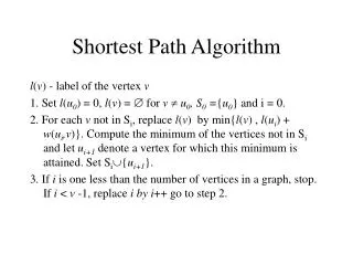
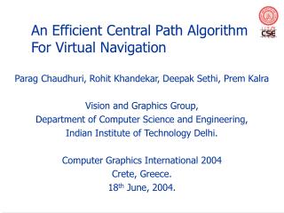
An Efficient Central Path Algorithm For Virtual Navigation
This paper presents an innovative algorithm for navigating three-dimensional closed objects, focusing on finding optimal paths that lie within the object, avoiding boundaries, and minimizing length. The proposed method uses hierarchical subdivision to compute a Distance From Boundary (DFB) field, allowing for efficient path computation using shortest path algorithms. The approach is applied in various applications, including virtual surgery, flight planning, and gaming. The algorithm demonstrates reduced computational complexity, with paths of varying resolutions and efficient handling of input scaling.

An Efficient Central Path Algorithm For Virtual Navigation
E N D
Presentation Transcript
An Efficient Central Path Algorithm For Virtual Navigation Parag Chaudhuri, Rohit Khandekar, Deepak Sethi, Prem Kalra Vision and Graphics Group, Department of Computer Science and Engineering, Indian Institute of Technology Delhi. Computer Graphics International 2004 Crete, Greece. 18th June, 2004.
Motivation • Navigation in virtual environments is needed in many applications such as • Virtual Surgery • Automatic flight planning • Computer games
The Problem • Given a three dimensional closed object and two points in the interior, find a path connecting those two points that • Lies completely inside the object • Stays away from the boundary • Has short length
Background • Topological thinning • Pavlidis 1980, Paik et. al. 1998, Ge et. al. 1999, Bouix et. al. 2003, Telea & Vilanova 2003 • Potential field based methods • Hong 1995, Deschamps & Cohen 2001 • Distance field based methods • Bitter et. al. 2001, Wan et. al. 2001
Distance From Boundary (DFB) • Distance of a point from the nearest boundary. • Different measures of distance – Euclidean, City-block, Champher. • Find a path such that sum of DFB field at all points on the path is maximized.
Our Approach • Compute DFB field for a hierarchical subdivision as opposed to computing DFB for the entire object at the finest resolution.
Hierarchical Subdivision • Enclose the object in a bounding box
Hierarchical Subdivision • Subdivide the box into four equal parts
Hierarchical Subdivision • Keep subdividing the smaller parts till they are intersecting with the boundary of the object.
Hierarchical Subdivision • The smallest size boxes are the voxels with size 1. • Size of a block b (size(b)) is the number of voxels on its side.
DFB Field Computation 1 2 4 8
DFB Field Computation • We compute the DFB for the cells by running a shortest path algorithm from the boundary to all the cells.
Path Computation • We can find the path between any two points by running a shortest path algorithm on the graph formed by the cells. • An edge between blocks b1 and b2 in the graph is now given a weight w as W(b1,b2)=1/dfb(b1)+1/dfb(b2)
Path Computation • The algorithm returns a path in terms of connected blocks.
Path Computation • A path is obtained by joining the centres of the blocks.
Path Smoothening Corner Cutting Splines
Result – Computational Complexity • It is proved that the number of voxels formed in the final subdivision are O(n+hk) • n : number of voxels on the boundary. • h : number of holes in the object. • k : number of levels of subdivision. • The running time is O((n+hk)log(n+hk))
The Progressive Algorithm • We usually do not need to compute the DFB for the entire object. • The extraneous volume for which the DFB is computed becomes a bottleneck at times.
The Progressive Algorithm • Subdivide the region into coarse grid. • Choose a Region Of Interest (ROI) which contains the source and destination. • Compute the path for this ROI.
The Progressive Algorithm • Grow the ROI and recompute the path. • Continue growing until the change in path length falls below a threshold.
Conclusion • DFB/Path computation is fast. • Paths of multiple resolutions. • Scaling the input does not adversely affect the computation time. • The subdivision grid also aids in View Culling while rendering. • Progressive extension makes it more efficient.