The Importance of Wave Acceleration and Loss for Dynamic Radiation Belt Models

1. The Importance of Wave Acceleration and Loss for Dynamic Radiation Belt Models Richard B. Horne M. M. Lam, N. P. Meredith and S. A. Glauert, British Antarctic Survey, Cambridge, UK R.Horne@bas.ac.uk 3rd European Space Weather Week Brussels, 14 November 2006

2. Rapid variations in radiation belt Damage spacecraft Hazard to astronauts Object To develop a dynamic radiation belt model Use of dynamic models To specify periods of risk To analyse events To determine extreme events To specify conditions where little (no) data is available CRRES ~1 MeV Electron Flux

3. Importance of Wave Processes • Structure of ‘quiet-time’ radiation belt controlled by losses due to waves • Lyons and Thorne [1973] • Losses due to lightning (whistlers), ground based transmitters, hiss • Abel and Thorne [1998a, b] • Losses due to microbursts precipitation (chorus waves) • Obrien et al. [2003] • Losses due to EMIC waves • Summers and Thorne [2005], Albert [2005] • Flux increases during 2003 Halloween due to chorus wave acceleration • Horne et al. Nature [2005], Shprits et al. [2006] • Wave acceleration on global scale • Varotsou et al. [2005], Horne et al. [2006]

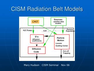
4. Radiation Belt Model • Solve the Fokker Planck equation in 1d • 1st term is transport across B (for constant 1st +2nd invariants J1, J2) • 2nd term is losses due to wave-particle interactions • Focus only on losses due to whistler mode hiss • Use BAS wave database and PADIE code to calculate losses • Use data at GEO and calculate flux near L=3-4 • GPS satellites • Galileo satellites

5. CRRES Data at L=6 • Note energy dependence in flux variations • Outer boundary condition requires flux at different energies

6. Conservation of adiabatic invariants (J1, J2) electrons accelerated when transported inward Inward Transport • At GEO - need observations at 0.05 – few MeV

7. Contribution of Wave-Particle Interactions: Which Waves?

8. Intensity of Whistler Mode Hiss • Wave intensity increases with Kp • Changes in high density plasmapause region is critical for wave power • Note plume region on dayside • Latitude: 5o – 30o

9. Hiss observed to 30o latitude Averaged over 06:00-21:00 MLT Include wave-particles interactions along magnetic field due to distribution of waves Latitude Coverage of Hiss

10. Assume Peak wave frequency at 550 Hz and width of 200 Hz Peak power in field aligned direction with 20o spread 10 harmonic resonances Bounce –average to mirror point Electron loss to atmosphere when diffusion rates are high near the loss cone (~ 4 degrees at L=4) Losses increase for fpe/fce small fpe/fce =2 purple Fpe/fce = 18 red E = 1 MeV L=4 Fpe/fce = 2, 6, 10, 14, 18 Pitch Angle Diffusion – PADIE Results

11. Pitch Angle Diffusion Matrix for Hiss

12. Model – Satellite Comparison - 1 MeV • Drive model by time series of Kp • Use flux at L=6 as outer boundary • Look up fpe/fce and wave power according to Kp • Scale diffusion matrix and obtain loss rates at all MLT • Solve Fokker-Planck eqn. and obtain flux CRRES Model

14. Radial diffusion only Radial diffusion and chorus waves Horne et al. [2006]

15. Conclusions • Model predicts MeV flux at L=3 – 4 from observations at L=6 using RD + wave losses • Losses inside plasmapause near L~4 are major importance • Predictions better than empirical models • Flux L>4 underestimated – suggests local acceleration required • Model improvements • Include wave acceleration outside plasmapause - chorus waves • Varotsou et al. [2005]; Horne et al [2006] • Include losses due to other waves modes • EMIC, chorus, whistlers, transmitters, magnetosonic waves • Data requirements • Electron flux at 0.1 – few MeV at GEO • Galileo and GPS data for verification at L~4 • Wave database with different wave modes

16. Timescale for Inward Transport • If flux at outer boundary drops by a factor of 100 for 10 days • Flux at L=4 responds after 2 days • If flux drops for only 1 day • Almost no response at L<4