Lectures 6&7: Image Enhancement
410 likes | 611 Views
Lectures 6&7: Image Enhancement. Professor Heikki Kälviäinen Machine Vision and Pattern Recognition Laboratory Department of Information Technology Faculty of Technology Management Lappeenranta University of Technology (LUT) Heikki.Kalviainen@lut.fi http://www.lut.fi/~kalviai

Lectures 6&7: Image Enhancement
E N D
Presentation Transcript
Lectures 6&7: Image Enhancement • Professor Heikki Kälviäinen • Machine Vision and Pattern Recognition Laboratory • Department of Information Technology • Faculty of Technology Management • Lappeenranta University of Technology (LUT) • Heikki.Kalviainen@lut.fi • http://www.lut.fi/~kalviai • http://www.it.lut.fi/ip/research/mvpr/ Prof. Heikki Kälviäinen CT50A6100
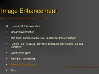
Content • Background. • Spatial domain methods. • Frequency domain methods. • Enhancement by point processing. • Spatial filtering. • Enhancement in the frequency domain. Prof. Heikki Kälviäinen CT50A6100
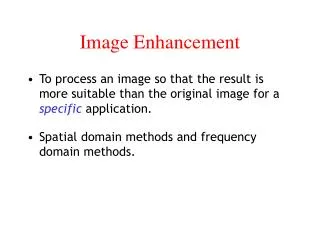
Background: Motivation • For preprocessing to make the image look better, i.e., more suitable for further processing. • Problems with • contrast, • sharpness, • smoothness, • noise, • distortions, • etc. Prof. Heikki Kälviäinen CT50A6100
Background: Spatial domain methods • Method: Slide the mask though the image and compute new pixel values. • Image processing function: • g(x,y) = T[f(x,y)] f(x,y) the input image g(x,y) the processed image T an operator on f, defined over some neighborhood of (x,y) • Gray-level transformation (mapping) function: • s = T(r) • r denotes f(x,y) and s denotes g(x,y) Prof. Heikki Kälviäinen CT50A6100
Background: Frequency domain methods • Method: Multiply the Fourier transforms of the image and the mask and apply the inverse transform to the multiplication. • Convolution: • g(x,y) = h(x,y)*f(x,y) • h(x,y) a linear, postion invariant operator • Fourier transform: • G(u,v) = H(u,v)F(u,v) • H(u,v) the transfer function of the process • Inverse Fourier transform: • g(x,y) = F^{-1} [H(u,v)F(u,v)] Prof. Heikki Kälviäinen CT50A6100
Enhancement by point processing: Some simple intensity transformations • Image negatives: • s = ((L-1) – r) where L = number of gray-levels • Contrast stretching: • Poor illumination, lack of dynamic range in the imaging sensor, wrong setting of a lens aperture during image acquisition. • To increase the dynamic range of the gray-levels. • Piecewise linear function. • When a thresholding function => a binary image (two values only). Prof. Heikki Kälviäinen CT50A6100
Contrast stretching Prof. Heikki Kälviäinen CT50A6100
Enhancement by point processing: Some simple intensity transformations (cont.) • Compression of dynamic range: • The dynamic range exceeds the capability of the display device. The need of brighter pixels. s = c log(1 + abs(r)) where c is a scaling constant • Gray-level slicing: • Highlighting a specific range of gray-levels with • “removing” or • preserving other pixels. Prof. Heikki Kälviäinen CT50A6100
Gray-level slicing • Original image (top). • Thresholded (left). • Gray-level slicing (right). Prof. Heikki Kälviäinen CT50A6100
Enhancement by point processing: Some simple intensity transformations (cont.) • Bit-plane slicing: • Select the specific bit planes. • For example: the image of eight 1-bit planes. • Plane 7 contains all the high-order bits: • Higher planes contain visually significant data. • Note: digital watermarking! • To select the plane 7 only corresponds to the image thresholded at gray-level 128. Prof. Heikki Kälviäinen CT50A6100
Enhancement by point processing: Histogram processing • Histogram of the image: • p(r_k) = n_k/n • where • r_k is the kth gray-level • n_k is the number of pixels with that gray-level • n is the total number of pixels in the image • k = 0, 1, 2, …, L-1 • L is the number of gray-levels Prof. Heikki Kälviäinen CT50A6100
Histogram of an image Prof. Heikki Kälviäinen CT50A6100
Enhancement by point processing: Histogram processing (cont.) • Histogram equalization (or histogram linearization): • to obtain the uniform histogram. • Gray-level transformation function and its inverse function: • s = T(r) • where 0<=T(r)<=1 and • T(r) is single-valued and monotonically increasing in 0<=r<=1 • r = T^{-1}(s) where 0<=s<=1 Prof. Heikki Kälviäinen CT50A6100
Histogram equalization Prof. Heikki Kälviäinen CT50A6100
Enhancement by point processing: Histogram processing (cont.) • Probability density function: • p_s(s) = [p_r(r) dr/ds]_{r=T^{-1}(s)} • Transformation function: • s = T(r) = integral_0^r (p_r(w)dw) • where 0<=r<=1 • ds/dr=p_r(r) • Uniform density • p_s(s) = [p_r(r) 1/p_r(r)]_{r=T^{-1}(s)} = 1 • where 0<=s<=1 • To obtain T^{-1} analytically is not always easy! Prof. Heikki Kälviäinen CT50A6100
Enhancement by point processing: Histogram processing (cont.) • Example: • p_r(r) = -2r + 2 when 0<=r<=1 • 0 elsewhere • What transformation function makes the uniform density? • s = T(r) = integral_0^r ((-2w + 2)dw) = -r^2 + 2r • Proof: • r = T^{-1}(s) = 1 ± sqrt(1-s), 0≤r≤1 => r = 1 - sqrt(1-s) • p_s(s)=[p_r(r)dr/ds] = [(-2r+2)dr/ds] = 1 0≤s≤1 Prof. Heikki Kälviäinen CT50A6100
Enhancement by point processing: Histogram processing (cont.) • In discrete form, probabilities: • p_r(r_k) = n_k/n • where 0≤r_k≤1 and k = 0, 1, …, L-1 • Transformation function: • s_k = T(r_k) = ∑ n_j/n j=0,...,k • = ∑ p_r(r_j) j=0,...,k • where 0≤r_k≤1 and k=0,1,…,L-1 • The new value n is the gray-level closest to the sum of probabilities up to the original value k: • n = round((L-1) x s_k) Prof. Heikki Kälviäinen CT50A6100
Enhancement by point processing: Histogram processing (cont.) • Histogram specification: • To apply another transformation function than an approximation to a uniform histogram. • Local enhancement: • Local processing instead of the whole image. • For example, histogram equalization of a 7x7 neighborhood about each pixel. Prof. Heikki Kälviäinen CT50A6100
Enhancement by point processing:Image subtraction • The difference between two images f(x,y) and h(x,y): • g(x,y) = f(x,y) – h(x,y) • done by pixelwise subtraction. • The use of the mask image. • Applications in medical image processing: • The mask is a normal image which is subtracted from a sample image to point out regions of interest. Prof. Heikki Kälviäinen CT50A6100
Image subtraction Prof. Heikki Kälviäinen CT50A6100
Enhancement by point processing:Image averaging • Consider a noisy image g(x,y) formed by the addition of noise η(x.y) to an original image image f(x,y): • g(x,y) = f(x,y) + η(x.y) • By averaging noisy images, noise is reduced. • Noise must be uncorrelated and must has the zero average value! • Example: noisy microscope images. Prof. Heikki Kälviäinen CT50A6100
Spatial filtering: Background • Spatial filtering: the use of spatial filters. • Spatial filters: • Lowpass filters. • Highpass filters. • Bandpass filters. • The mask: w1 w2 w3 • w4 w5 w6 • w7 w8 w9 • Smoothing filters, sharpening filters. Prof. Heikki Kälviäinen CT50A6100
Spatial filtering: Smoothing filters • For blurring and noise reduction. • Lowpass spatial filtering: 1 1 1 1/9 x 1 1 1 1 1 1 • Neighborhood averaging. • Median filtering: replace the gray-level of each pixel by the median of the gray-levels in a neighborhood of that pixel. • Removes noise, but preserves details such as edges. • Filter size?, weighted median filtering? Prof. Heikki Kälviäinen CT50A6100
Spatial filtering: Averaging vs. median • Original image (upper left). • Original + noise (upper right). • Smoothed image (lower right). • Median smoothing (lower left). Prof. Heikki Kälviäinen CT50A6100
Spatial filtering: Sharpening filters • For highlighting fine detail in an image or enhance detail that has been blurred. • Filters: • Basic highpass spatial filter. • High-boost filtering. • Derivative filters. Prof. Heikki Kälviäinen CT50A6100
Spatial filtering: Basic highpass spatial filtering • Positive coefficients near the center of a filter, negative coefficients in the outer periphery. • 3 x 3 sharpening filter: • -1 -1 -1 • 1/9 x -1 8 -1 • -1 -1 -1 • The sum of the coefficients is zero. • The filter eliminates the zero frequency term => • the reduced global contrast of the image. • Scaling and/or clipping for negative values to map the range [0, L-1]. Prof. Heikki Kälviäinen CT50A6100
Spatial filtering: High-boost filtering • Highpass = Original – Lowpass. • High-boost or high-frequency-emphasis filter: • High boost = (A)(Original) – Lowpass • = (A-1)(Original) + Original – Lowpass • = (A-1)(Original) + Highpass. • Looks like an original image, with edge enhancement by A. Prof. Heikki Kälviäinen CT50A6100
Spatial filtering: High-boost filtering (cont.) • Unsharp masking: to subtract a blurred image from an original image. • In the printing and publishing industry. • The mask with w = 9A -1 (with A≥1): • -1 -1 -1 • 1/9 x -1 w -1 • -1 -1 -1 Prof. Heikki Kälviäinen CT50A6100
Spatial filtering: Derivative filters • For sharpening an image (averaging vs. differentiation). • The gradient of f(x,y): • ∂f/∂x • df = • ∂f/∂y • The magnitude is the basis for image differentiation methods: • mag(df)= ((∂f/∂x)^2 + (∂f/∂y)^2)^(-1/2) Prof. Heikki Kälviäinen CT50A6100
Spatial filtering: Derivate filters (cont.) • Roberts: 1 0 0 1 • 0 -1 1 0 • Prewitt: • -1 -1 -1 -1 0 1 • 0 0 0 -1 0 1 • 1 1 1 -1 0 1 • Sobel: • -1 -2 -1 -1 0 1 • 0 0 0 -2 0 2 • 1 2 1 -1 0 1 Prof. Heikki Kälviäinen CT50A6100
Enhancement in the frequency domain • The use of image frequencies for enhancement. • Convolution: f(x)*g(x) F(u) G(u). • The filtered image g(x,y) using the Fourier transforms of an original image f(x,y) and a mask h(x,y): • g(x,y) = F^{-1} [H(u,v)F(u,v)] • Lowpass filtering. • Highpass filtering. Prof. Heikki Kälviäinen CT50A6100
Images and Their Fourier Spectra F(k) also denoted F(u) i = sqrt(-1) F(x,y) also denoted F(u,v) Prof. Heikki Kälviäinen CT50A6100
Discrete Fourier Transform (DFT) Prof. Heikki Kälviäinen CT50A6100
Fourier transform: Image power Distance from point (u,v) to the origin: D(u,v) = ((u^2 + v^2))^(-1/2) • Radius (pixels) % Image power • 8 95 • 16 97 • 32 98 • 64 99.4 • 128 99.8 Prof. Heikki Kälviäinen CT50A6100
Enhancement in the Frequency Domain: Lowpass filter • G(u,v) = H(u,v) F(u,v). • Ideal lowpass filter: • H(u,v) = 1 if D(u,v) ≤ D_0, or 0 if D(u,v) > D_0. • Original (left) and filtered image (right). Prof. Heikki Kälviäinen CT50A6100
Enhancement in the Frequency Domain: Butterworth lowpass filter • The transfer function: • H(u,v) = 1/(1 + (D(u,v)/D_0)^(2n)) • where • n is the order of the filter • D_0 is the cutoff frequency locus (select!) • H(u,v) from 1 to 0. • When D(u,v) = D_0, H(u,v) = 0.5. • H(u,v) = 1/√2 commonly used. Prof. Heikki Kälviäinen CT50A6100
Enhancement in the Frequency Domain: Highpass filter • Ideal high pass filter: • H(u,v) = 0 if D(u,v) ≤ D_0, or 1 if D(u,v) > D_0. • Original (left) and filtered image (right). Prof. Heikki Kälviäinen CT50A6100
Enhancement in the Frequency Domain: Butterworth highpass filter • The transfer function: • H(u,v) = 1/(1 + (D_0/D(u,v))^(2n)) • where • n is the order of the filter • D_0 is the cutoff frequency locus • H(u,v) from 0 to 1. • When D(u,v) = D_0, H(u,v) = 0.5. • H(u,v) = 1/√2 commonly used. Prof. Heikki Kälviäinen CT50A6100
Summary • For preprocessing to make the image look better, i.e., more suitable for further processing. • Approaches: • Spatial domain methods. • Frequency domain methods. • Enhancement by point processing. • Spatial filtering. • Enhancement in the frequency domain. Prof. Heikki Kälviäinen CT50A6100