Download
1 / 41
410 likes | 661 Views
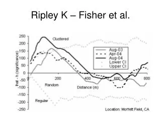
Ripley K – Fisher et al. Ripley K - Issues. Assumes the process is homogeneous (stationary random field). Ripley K was is very sensitive to study area size. Riley K is influenced by study area shape, the expected L(d) assumes a simple geometry.

E N D
Ripley K - Issues • Assumes the process is homogeneous (stationary random field). • Ripley K was is very sensitive to study area size. • Riley K is influenced by study area shape, the expected L(d) assumes a simple geometry. • Ripley K has strong basis near the edge/boundary. You should use a boundary correction method, and if your study area is not a simple shape you should use study are polygon. • Weighting points
Boundary Correction Methods • Boundary Correction Methods • RIPLEY EDGE CORRECTION FORMULA • SIMULATE OUTER BOUNDARY VALUES • REDUCE ANALYSIS AREA • Study Area Method • MINIMUM ENCLOSING RECTANGLE • USER PROVIDED STUDY AREA
Point Transformations • In many situations we collect “point” measurements of an entity we wish to study, but prefer/need to have an area (i.e. polygon) or field (e.g. raster) representation to relate the measurements to other information or have information at locations not measured to make decisions.
Four Basic Types of Methods • Point to Area Transformations (Deterministic) • Delineate areas and assign the point measurement(s) to the area. An Area is related to one or more points • Points are usually weighted. • Density Mapping – point to field (Deterministic) • A field element (e.g. a raster cell) is assigned a value based on sampling the surrounding neighborhood and computing the “density” of observations around the element. Density is the quantity per area. • Points can weighted or un-weighted.
Four Basic Types of Methods • Interpolation Methods – point to field (Deterministic) • A field element is assigned a value based on a mathematical transformation that predicts what the value should be at the field element location based on known point observations. • Points must be weighted. • Local Interpolation Methods • Uses a sub-sample of point observations to develop the mathematical equation and make the prediction. • Global Interpolation Methods • Uses all the point observations to develop the mathematical equation. Regression and trend analysis are examples. • Stochastic Modeling – field generation (Stochastic) • Use point observations to understand the statistical properties of an entity and to develop a model that generates a field of values that retain the statistical properties of the entity.
Point to Area Transformations Data Rasterization Voronmoi Polygons Zone of Influence Irregular Polygons Zone/Vornomoi
Point to Area Transformation Methods • Voronmoi (Thiessen) Polygons • The most commonly used. • Based on the concept of Nearest Neighbor. • Creates (usually) unequal size areas around each point. The areas are assigned the value of the origin point. • Depending on the distribution of points the range in sizes can be relatively large, but the entire analysis area is covered.
Thiessen Polygons • The Thiessen polygons are constructed as follows: All points are triangulated into a triangulated irregular network (TIN) that meets the Delaunay criterion. The perpendicular bisectors for each triangle edge are generated, forming the edges of the Thiessen polygons. The location at which the bisectors intersect determine the locations of the Thiessen polygon vertices.
Point to Area Transformation Methods • Irregular Shaped Polygons • Based on modeling or analysis, sometimes using additional data. • Watershed Delineation • Need outlet point and surface representation (e.g. DEM). • Model flow across surface to outlet point. • All areas that flow to outlet point are in watershed. • Minimum Convex Polygons (MCP) • Minimum area around all selected points. • Can create MCP that contain a percentage of the points.
Minimum Convex Polygon Hawth's Analysis Tools is an extension for ESRI's ArcGIS http://spatialecology.com
Density Mapping • Also referred to as Intensity. • Point to field raster data structure • Calculates the density of points in a neighborhood around each output grid cell. Neighbor is usually larger then the cell. • Points can be weighted (using a numeric attribute) or un-weighted (all points = 1). • Units of density are quantity per unit area. • Good for when the density of points is small relative to the desired cell size. • Two methods – Simple and Kernel.
Simple Density Mapping • The density is calculated using the number of points that fall within the neighborhood of each output grid cell, divided by the area of the neighborhood. For a circle neighborhood the equation is: n D(s) = (si / 2) hi <= i=1 where: D(s) = density (intensity) at point s (grid cell center) si = observation point i (equals 1 or a quantity) = radius of circle neighborhood hi = Euclidean distance between point and cell center. n = number of observations points within the neighborhood
Simple Density Mapping • Rough surfaces, all points have the same weight within search radius regardless of distance. • No assumptions regarding the kernal method type. • Called Point Density in ArcMap. • Can use different neighborhood shapes: • Circle (most common) • Rectangle • Wedge • Annulus
Kernel Density Mapping • A kernel function is used to fit a smoothly tapered surface to each point, and the density is calculated from these surfaces where they overlap the center of the output grid cell. This gives a smoother output grid, while maintaining the same general values for density. A circular neighborhood is always used with the KERNEL option.
Kernel Density Function • There are several commonly used kernel functions: • Gaussian • Quadratic(in ESRI) • Uniform • Triangle
Kernel Density Mapping • ArcGIS uses a quadratic kernel function where: n D (s) = si (3/2) [1 – (hi2/2)]2 hi <= i=1 D(s) = 0 otherwise where: = radius of circle neighborhood hi = distance between the point s and the observation point si n = number of observation points D(s) = density (intensity) at point s (grid cell center) si = observation point i (equals 1 or a quantity)
Kernel Density Mapping • Assume = 10m; si = 1; with 5 points • If hi = 0: D(si) = si * (3/2) * 1.0000 = 0.0095 • If hi = 2: D(si) = si * (3/2) * 0.9216 = 0.0088 • If hi = 5: D(si) = si * (3/2) * 0.5625 = 0.0054 • If hi = 7: D(si) = si * (3/2) * 0.2601 = 0.0025 • If hi = 9: D(si) = si * (3/2) * 0.0361 = 0.0003 • D(S) = 0.0265 units per square meter • If all points hi = 9: D(S) = 0.0015 units per sq. m. • D(S)simple = 5 / 2 = 5 /314.159 m2 = 0.0159 units per sq. m.
Kernel Density Mapping • Factors that influence surface characteristics: • Method: Simple would have a rougher looking surface, but typically less variance. • Neighborhood Size: the greater the number of points used to compute density the less variance in the surface. • Cell Size: the larger the cell the rougher, greater potential relative change per cell. • You can made a surface to smooth and loss the natural variance of the surface, areas with high and low density. • You should experiment, what creates the “best” surface for you. Some use the search distance where variance starts to become stable.
Density Mapping Kernel, Radius = 10 CellSize = 5x5m Mean = 0.0094 S.D. = 0.0073 Kernel, Radius = 20 CellSize = 5x5m Mean = 0.0088 S.D. = 0.0038
Density Mapping Kernel, Radius = 20 CellSize = 2x2m Mean = 0.0088 S.D. = 0.0038 Kernel, Radius = 20 CellSize = 5x5m Mean = 0.0088 S.D. = 0.0038
Density Mapping Kernel, Radius = 20 CellSize = 2x2m Mean = 0.0088 S.D. = 0.0038 Simple, Radius = 20 CellSize = 2x2m Mean = 0.0083 S.D. = 0.0031
20m 40m 10m 15m Density Mapping Patchy Trend
Density surface using bivariate normal density kernel This figure is a display of the location points (shown in yellow) within the selected 50, 75, and 90% probability polygons.
Here is a kernel density map of the cholera deaths (kernel size = 1.0; cellsize = 0.0025) with density contours overlaid. The density of cholera deaths derived from this map is 36.8 at the Broad Street pump, versus 2.4 at Carnaby Street, 1.9 at Rupert Street, 0.8 at Marlborough Mews, 0.2 at Bridle Street, 0.1 at Newman Street and zero at all other pumps. A simple density analysis with no smoothing yielded a similar map with discrete edge segments.
Interpolation • Global Interpolation Methods • Trend Analysis (Global Polynomials) • Regression (spatial and non-spatial)
Interpolation • Trend Analysis • Surface is approximated by a polynomial • Value (z) at any point (x,y) on the surface is given by an equation in powers of x and y. • Linear equation (1 degree) describes a tilted plane surface • z = a + bx + cy • Quadratic equation (2 degree describes a simple hill or valley • z = a + bx + cy + dx2 + exy + fy2
Interpolation • Trend Analysis • In general, any cross-section of a surface of degree n can have at most n-1 alternating maxima and minima. • Assumes the general trend of the surface is independent of random errors found at each sample point. • Good at addressing non-stationary cases.