Download
1 / 19
190 likes | 382 Views
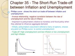
The Short-Run Trade-Off Between Inflation and Unemployment. Chapter 5. Philips Curve. Phillips curve : shows the short-run trade-off between inflation and unemployment 1958: A.W. Phillips showed that nominal wage growth was negatively correlated with unemployment in the U.K.

E N D
The Short-Run Trade-Off Between Inflation and Unemployment Chapter 5
Philips Curve • Phillips curve: shows the short-run trade-off between inflation and unemployment • 1958: A.W. Phillips showed that nominal wage growth was negatively correlated with unemployment in the U.K. • 1960: Paul Samuelson & Robert Solow found a negative correlation between U.S. inflation & unemployment, named it “the Phillips Curve.”
So What? • “The Phillips curve shows the combinations of inflation and unemployment that arise in the short run as shifts in the aggregate-demand curve move the economy along the short-run aggregate supply curve” (803).
P inflation SRAS B B 5% 105 A A 103 AD2 3% PC AD1 Y 6% u-rate 4% Y2 Y1 Example: • PL=100 in 2020 • Two outcomes are possible in 2021 • If AD is high… PL rises by a lot (output increases substantially) (B) • If AD is low… PL rises by a little (output increases slightly) (A)
Analysis of the graphs: • Both graphs are connected • As “A” moves to “B” the output increases • Higher output= higher demand for workers • Higher demand for workers= lower unemployment • As “A” moves to “B” the PL increases • Increasing the PL increases the rate of Inflation
Shifts in the Philips Curve: The Role of Expectations • Fiscal and monetary policies affect the AD; therefore, the PC offers policymakers a menu of choices: • low unemployment with high inflation • low inflation with high unemployment • anything in between
The Vertical Long-Run Phillips Curve • Natural-rate hypothesis: the claim that unemployment eventually returns to its normal or “natural” rate, regardless of the inflation rate • Based on the classical dichotomy and the vertical LRAS curve
P Inflation LRAS LRPC P1 P2 AD2 high inflation low inflation AD1 Y u-rate Natural rate of output Natural rate of unemployment Therefore…
Graph Analysis: • Since the LRAS curve is vertical, and output stays constant, any increase in AD just increases Inflation.
Quick Vocabulary: • Expected Inflation: • Measure of how much people expect the overall PL to change
The Phillips Curve Equation: • Unemployment Rate (UR) • Natural Rate of Unemployment (NRU) • Actual Inflation (AI) • Expected Inflation (EI) UR= NRU+ a(AI – EI) a= in a parameter of how much unemployment responds to unexpected inflation
Answers: Short run Fed can reduce u-rate below the natural u-rate by making inflation greater than expected. Long runExpectations catch up to reality, u-rate goes back to natural u-rate whether inflation is high or low.
Quick Vocabulary: • Natural-Rate Hypothesis: • Claims that unemployment eventually returns to its normal, or natural, rate, regardless of the rate of inflation
Another PC Shifter: Supply Shocks • Supply shock: an event that directly alters firms’ costs and prices, shifting the AS and PC curves • Example: large increase in oil prices
P Inflation SRAS2 SRAS1 B B P2 A A P1 PC2 AD PC1 Y U-Rate Y1 Y2 Effects of Supply Shock:
Graph Analysis: • SRAS Curve shifts left: • Output decreases • Price level increases • Unemployment rises
Costs of Reducing Inflation: • Sacrifice Ratio: • The number or % points of annual output lost in the process of reducing inflation by 1% point • Rational Expectations: • The theory that people optimally use all the information they have including information about gov.t policies, when forecasting the future
Costs of Reducing Inflation: (Sacrifice ratio) • Typical estimate of the sacrifice ratio: 5 • To reduce inflation rate 1%, must sacrifice 5% of a year’s output. • Can spread cost over time, e.g. To reduce inflation by 6%, can either • sacrifice 30% of GDP for one year • sacrifice 10% of GDP for three years
Costs of reducing Inflation:(Rational Expectations) • Ex. • Fed claims that they’re going to reduce inflation • Expected Inflation decreases (SRPC shifts downward) • Result: • Disinflations can cause less unemployment that the traditional sacrifice ratio predicts.