Download
1 / 8
80 likes | 330 Views
Multiple Altimeter Beam Experimental Lidar (MABEL) First Flights and Initial Results. Matthew McGill, Code 613.1, NASA GSFC. MABEL was developed as a demonstrator and validation tool for the ICESat-2 photon-counting altimetry concept.

E N D
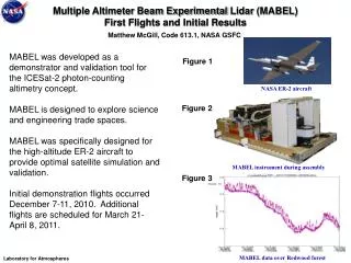
Multiple Altimeter Beam Experimental Lidar (MABEL) First Flights and Initial Results Matthew McGill, Code 613.1, NASA GSFC MABEL was developed as a demonstrator and validation tool for the ICESat-2 photon-counting altimetry concept. MABEL is designed to explore science and engineering trade spaces. MABEL was specifically designed for the high-altitude ER-2 aircraft to provide optimal satellite simulation and validation. Initial demonstration flights occurred December 7-11, 2010. Additional flights are scheduled for March 21-April 8, 2011. Figure 1 NASA ER-2 aircraft Figure 2 MABEL instrument during assembly Figure 3 MABEL data over Redwood forest Laboratory for Atmospheres
Name: Matthew McGill, NASA/GSFC E-mail: Matthew.J.McGill@nasa.gov Phone: 301-614-6281 Background: The Multiple Altimeter Beam Experimental Lidar (MABEL) was developed to conclusively demonstrate the ICESat-2 photon-counting altimetry concept. The instrument was designed to explore science and engineering trade spaces, including (1) variable beam spacing/pattern; (2) variable laser repetition rate; (3) two wavelength (532 and 1064 nm) operation; (4) variable energy per footprint. Completed in just 12 months, the first flights occurred December 7-11, 2010. Technical Description of Images: Figure 1: The NASA ER-2 high-altitude research aircraft. The MABEL instrument was specifically designed for this high-altitude platform to provide the best possible satellite simulation capability. Research altimeters flying at lower altitudes do not mimic the ICESat-2 viewing geometry and are not complicated by having intervening atmosphere between the sensor and the surface. Figure 2: The MABEL instrument, as built. Built in 12 months, concept-to-flight, MABEL is an engineering success. Relevant instrument parameters include: • operational altitude: 20 km • wavelength: 532 and 1064 nm • telescope diameter: 6 inches • laser footprint diameter: 100 rad (2 m) • telescope field of view: 210 mrad (4.2 m) • sampling width: +/- 1.05 km (max) • 16 simultaneous footprints at 532 nm; 8 simultaneous footprints at 1064 nm Figure 3: Data from MABEL over a Redwood forest in the Sierra Nevadas, December 10, 2010. The image shows a single channel. The forest is coniferous and not completely dense. Ground return is easily observed between trees. Tree height was verified using an interpolated global vegetation grid. Scientific significance: MABEL demonstrates conclusively that the photon-counting altimetry concept is a valid measurement approach for the ICESat-2 mission. Analysis of MABEL data over varying surfaces will provide verification of ICESat-2 measurement requirements. Relevance for future science and relationship to Decadal Survey: As a demonstrator for ICESat-2, the MABEL instrument has shown the measurement concept is sound. Future science flights will focus on ice and snow measurements, and ultimately, post-launch validation of the ICESat-2 mission. Laboratory for Atmospheres
Comparing the ENSO and Volcanic Effects on the Global Water CycleGuojun Gu and Robert F. Adler, Code 613.1, NASA/GSFC & ESSIC/University of Maryland • Global water and energy cycles may respond differently to distinct climatic perturbations such as ENSO and volcanic eruptions. Using satellite observations, variations associated with ENSO and volcanic eruptions are identified in several key physical components and further compared in their global and tropical fields. • ENSO related anomalies are evident in zonal-mean precipitation, surface and tropospheric temperatures, and columnar water vapor especially during the major ENSO events (for instance, the 97/98 event), though they manifest distinct meridional structures. • No coherent ENSO anomalies are discovered in mid-lower tropospheric static instability (TLT-TMT). However, TLT-TMT shows strong responses to volcanoes and an increasing trend especially in the mid-higher latitudes. • ENSO signals in temperatures and water vapor remain strong when integrated over both the tropics and the globe, while the ENSO related precipitation signals in general become muted, consistent with the negligible TLT-TMT signals. • For volcanoes, the strong signals are seen in the time series of not only temperatures and water vapor, but also precipitation and TLT-TMT. P Ts CWV TLT TMT TLT-TMT Pinatubo El Chichon Figure 1Time-latitude diagrams of zonal-mean anomalies of precipitation (P), surface temperature (Ts), columnar water vapor (CWV), lower-tropospheric temperature (TLT), middle-tropospheric temperature (TMT), and TLT-TMT. Figure 2Time series of global mean (a) Ts, (b) CWV, (c) P, (d) TLT, (e) TMT, and (f) TLT-TMT. Also shown are their corresponding ENSO (red lines) and volcanic (green lines) responses. Laboratory for Atmospheres
Name: Guojun Gu, NASA/GSFC, Code 613.1 and ESSIC/University of Maryland E-mail: Guojun.Gu-1@nasa.gov Phone: 301-614-6337 Reference: Gu, G., and R. F. Adler, 2011: Precipitation and temperature variations on the interannual time scale: Assessing the impact of ENSO and volcanic eruptions. Journal of Climate, DOI: 10.1175/2010JCLI3727.1. (in press) Data Sources: Monthly rain-rates from the Global Precipitation Climatology Project (GPCP), global surface temperature anomalies from the NASA-GISS temperature anomaly analysis, SSM/I-RSS oceanic columnar water vapor content, columnar water vapor content over land from NASA/MERRA, and MSU/AMSU lower tropospheric and mid-tropospheric temperatures. Technical Description of Figures: Mean seasonal cycles in various components are first removed at each grid point. Time-latitude maps of zonal-mean anomalies are then constructed by integrating over the entire longitude band. The time series of global (and tropical) means for these variables are also constructed. Nino 3.4, a time series of sea surface temperature (SST) anomalies averaged over a domain of 5oN-5oS, 120-170oW in the tropical Pacific, is used to represent the ENSO events. Volcano eruptions (El Chichón, March 1982; Mt. Pinatubo, June 1991) are denoted by the tropical mean stratospheric aerosol optical thickness (). The GPCP time span (January 1979-December 2008) is divided into two periods based on the monthly magnitude of . One period has a volcanic impact (defined as 0.016), while the other period is the remainder of the time span ( 0.016). The ENSO effects are estimated during the non-volcanic period using lag-correlation/regression analyses, which are further applied to the volcano period. Once the ENSO signals are identified and removed in the time series, volcanic signals if any, are then estimated using lag-correlation/regression analyses. The ENSO and volcano effects are thus quantified. Figure 1: Time-latitude diagrams of zonal-mean anomalies of precipitation (P), surface temperature (Ts), columnar water vapor (CWV), lower-tropospheric temperature (TLT), middle-tropospheric temperature (TMT), and TLT-TMT. Figure 2: Time series of global mean (a) Ts, (b) CWV, (c) P, (d) TLT, (e) TMT, and (f) TLT-TMT. Also shown are their corresponding ENSO (red lines) and volcanic (green lines) responses. Scientific significance: This observational study improves our understanding of how and why the global water (and energy) cycle, specifically global precipitation and tropospheric water vapor content, responds differently to ENSO and volcano-related climatic perturbations. The results aid in interpreting global warming related processes/features which may already have happened in the past three decades. Relevance for future science and relationship to Decadal Survey: The study is the first step for assessing our current knowledge of global climate changes specifically in the global water cycle. It is further applicable to examining the capability of the state-of-the-art general circulation models (GCMs) in simulating these changes and to providing a check on GCM-based climate projections. Laboratory for Atmospheres
Near-cloud changes impact global aerosol statistics A. Marshak, T. Várnai, W. Yang, G. Wen, Code 613.2, NASA GSFC How do aerosol particles change in the vicinity of clouds? Figure 1 shows that areas near clouds occupy a large segment of all clear-sky regions, which implies that understanding aerosols near clouds is essential for understanding the role of aerosols in our climate. Comparison of the two panels in Figure 2 reveals that NASA’s CALIPSO lidar observes both stronger light scattering and increased particle size near clouds. (Particle size is closely related to color ratio.) The increases arise from processes such as aerosol particles swelling up in the humid air that surrounds clouds. Figure 3 shows that the increase in particle scattering is substantial and typically exceeds 40% within 5 km of clouds. The finding that particle changes in the transition zone are sufficiently prevalent to impact even global statistics highlight the importance of better understanding of these changes, and considering them both in the interpretation of satellite data and in climate simulations. The ultimate goal is to help reduce some of the largest sources of uncertainties in understanding human impacts on climate: aerosol-cloud inter-actions and aerosols reflecting or absorbing sunlight. Color ratio Far from clouds (> 5km) Close to clouds (< 5km) Fraction of clear areas that are closer to clouds than the distance D Log10 of 532 nm backscatter Number of cloud-free vertical profiles Distance (D) to nearest cloud (km) Figure 1: Fraction of clear-sky areas that are closer than a certain distance to clouds, based on MODIS and CALIPSO data. The inset illustrates that even in clear areas, clouds are rarely far away. Figure 2: Histograms of cloud-free CALIPSO lidar shots. The crossings of black lines point out where the left panel histogram peaks. A comparison of the two panels reveals that particle backscatter and size increase simultaneously near clouds. Backscatter characterizes light scattering and is closely related to the amount of aerosols. Figure 3: Median relative increase (Ra) of CALIPSO vertically integrated particle backscatter near clouds, over the value observed 20 km away. Laboratory for Atmospheres
Name: Alexander Marshak, NASA/GSFC Code 613.2E-mail: alexander.marshak@nasa.govPhone: 301-614-6122 References: Várnai, T., and A. Marshak, 2011: Global CALIPSO observations of aerosol changes near clouds. IEEE Geosci. Remote Sens. Lett., 8, 19-23. Várnai, T., and A. Marshak, 2009: MODIS observations of enhanced clear sky reflectance near clouds. Geophys. Res. Lett., 36, L06807, doi:10.1029/2008GL037089. Yang W., A. Marshak, T. Várnai, and Z. Liu, 2011. Effect of CALIPSO cloud aerosol discrimination (CAD) confidence levels on the observation of aerosol properties near cloud. IEEE Trans. Geosci. Remote Sens., (submitted Nov 2010). Data Sources: CALIPSO and MODIS Level 1 observations, and CALIPSO and MODIS Level 2 aerosol and cloud products. Technical Description of Figures: Figure 1: Cumulative histogram of clear-sky areas over all oceans, as a function of distance to the nearest cloud. Red curve is based on MODIS data for 9/21/2008 and considers all clouds, whereas the blue dashed curve is based on a month of CALIPSO data (9/15-10/14, 2008) and considers nearby clouds only if their top is below 3 km. The inset illustrates that even in clear areas, clouds are rarely far away. Figure 2: Histograms of CALIPSO lidar shots as a function of vertically integrated values of 532 nm backscatter (horizontal axis) and color ratio (vertical axis). The color ratio (the ratio of backscatters at 1064 nm and 532 nm) is related to particle size, with higher color ratios indicating larger particles. The crossing of black lines points out the location where the left panel histogram peaks. The comparison of the left panel (areas near clouds) and right panel (areas far from clouds) reveals that particle backscatter and size tend to increase simultaneously near clouds. Vertical integration is from the surface to 3 km altitude. Figure 3: Medians of the ratio (Ra) by which the vertically integrated particle backscatter values measured by the CALIPSO lidar increase near clouds, relative to the median particle backscatter observed 20 km away from clouds. The plot is based on the same dataset as Fig. 2 and the blue curve in Fig. 1. Scientific significance: Our results provide the first observational evidence of near-cloud particle changes being sufficiently strong to alter global statistics of aerosol populations. Due to physical processes such as swelling in humid air, aerosol particles change in a such wide transition zone around clouds that covers over half of all clear-sky areas. Because aerosol radiative impacts and aerosol-cloud interactions are major sources of uncertainty in understanding human impacts on climate, the prevalence of a wide and well-pronounced transition zone indicates a strong need for better understanding the particle changes near clouds. This implies that, despite remote sensing challenges such as cloud detection uncertainties or cloud adjacency effects, it is important to obtain accurate satellite measurements of aerosol properties near clouds. Relevance for future science and relationship to Decadal Survey: Better understanding aerosol radiative effects and aerosol-cloud interactions is critical for reducing uncertainties regarding human impacts on climate. The importance of studying this interaction is highlighted in the Decadal Survey and is a goal for future NASA missions such as ACE. Laboratory for Atmospheres
The Response of Tropical Tropospheric Ozone to ENSOLuke Oman, Jerry Ziemke, Anne Douglass, Jose Rodriguez, Code 613.3, NASA GSFC El Niño Southern Oscillation (ENSO) is the dominant mode of tropical variability on interannual timescales. Its influence extends beyond the thermal and dynamical and into the chemical composition of the troposphere. Ziemke et al. [2010] found a dipole in tropospheric column ozone between the western and eastern Pacific region. The Niño 3.4 Index (blue curve) from sea surface temperature anomalies is very well correlated to the difference between western and eastern Pacific ozone columns (black curve). Ziemke et al. [2010] identify this difference as an Ozone ENSO Index. An Ozone ENSO Index (OEI) computed using the Goddard Earth Observing System (GEOS) version 5 chemistry-climate model (CCM) reproduces the observed OEI. Observed sea surface temperatures are used in the simulation; natural and pollutant emission sources are repeated annually. We conclude that observed sea surface temperatures are dominant in driving the variability that controls this index. Figure 1:Comparison of GEOS CCM simulated (red curve) and a measurement derived (black curve) Ozone ENSO Index (OEI) with Niño 3.4 Index (multiplied by 3, blue curve) for the 1985 to 2009 time period. Laboratory for Atmospheres
Name: Luke Oman, NASA/GSFC, Code 613.3 E-mail: luke.d.oman@nasa.gov Phone: 301-614-6032 References: Ziemke, J.R., S. Chandra, L.D. Oman, and P.K. Bhartia (2010), A new ENSO index derived from satellite measurements of column ozone. Atmos. Chem. Phys., 10, 3711-3721. Oman, L.D, J.R. Ziemke, A.R. Douglass, D.W. Waugh, C. Lang, J.M. Rodriguez, and J.E. Nielsen (2011), The Response of Tropical Tropospheric Ozone to ENSO. Geophys. Res. Lett., in preparation. Data Sources: Nimbus 7 Total Ozone Mapping Spectrometer (TOMS), National Oceanic and Atmospheric Administration (NOAA) 9 Solar Backscatter Ultraviolet (SBUV/2), Earth Probe TOMS, and the Aura Ozone Monitoring Instrument (OMI) and Microwave Limb Sounder (MLS). Technical Description of Figures: Figure 1: The Ozone ENSO Index (OEI) is derived by averaging monthly tropospheric column ozone over two broad regions of the western and eastern Pacific (15°S-15°N, 70°E-140°E, and 15°S-15°N, 110°W-180°W, respectively) and taking their difference (western minus eastern Pacific). The time series is then deseasonalized and smoothed with a 3-month running average (black curve). We used the Goddard Earth Observing System (GEOS) version 5 coupled to the comprehensive Global Modeling Initiative (GMI) stratosphere-troposphere chemical mechanism to simulate the impact of observed sea surface temperature changes on tropospheric ozone concentrations. This simulation used fixed in time natural and anthropogenic emission sources to evaluate the variability due to sea surface temperature changes. Using the tropospheric column ozone amounts from the simulation averaged over the same two regions the values were differenced, deseasonalized, and smoothed using a 3-month running average (red curve). Niño 3.4 Index is shown as the blue curve multiplied by 3 for scaling. All three times series are strongly correlated over the 25 year period with Measurement vs. ENSO correlation of 0.84 and Simulation vs. ENSO correlation of 0.86. Scientific significance: The El Niño Southern Oscillation (ENSO) is the dominant mode of tropical variability on interannual timescales. It is well known to have significant influence on the Walker Circulation in the tropical Pacific. This work demonstrates the fundamental physical relationship between tropical sea surface temperatures anomalies and ozone distribution changes in the tropical troposphere. The OEI is derived using tropospheric column ozone measurements but important information about the vertical contributions to the tropospheric column change require ozone profile information like those provided in SHADOZ ozonesondes and MLS measurements in the upper troposphere. The work of Ziemke et al. [2010] is an important step toward viewing tropospheric ozone variability in a climate based context rather then as individual case studies. This OEI also provides an excellent measure of chemistry-climate models response to ENSO variability and can be used in their evaluation. Relevance for future science and relationship to Decadal Survey: A continuation of the long climate record (since 1979) of total and tropospheric column ozone is necessary with measurements from NASA’s AURA satellite using instruments like OMI and MLS. Future missions like the proposed Global Atmospheric Composition Mission (GACM) which will measure total column ozone as well as the vertical profile of ozone distribution especially in the upper troposphere and lower stratosphere will be very important in examining the vertical structure of these changes. Laboratory for Atmospheres