Download

1 / 23
230 likes | 387 Views
Matching and Recognition in 3D. Moving from 2D to 3D. Some things harder Rigid transform has 6 degrees of freedom vs. 3 No natural parameterization (e.g. running FFT or convolution is trickier) Some things easier No occlusion (but sometimes missing data instead)

E N D
Moving from 2D to 3D • Some things harder • Rigid transform has 6 degrees of freedom vs. 3 • No natural parameterization (e.g. running FFT or convolution is trickier) • Some things easier • No occlusion (but sometimes missing data instead) • Segmenting objects often simpler
Matching / Recognition in 3D • Methods from 2D • Feature detectors • Histograms • PCA (eigenshapes) • Graph matching, interpretation trees
Matching / Recognition in 3D • Other methods (may also apply to 2D) • Identifying objects in scene: spin images • Finding a single object in a database:shape distributions • Aligning pieces of the same object:iterative closest points (ICP)
3D Identification Using Spin Images • Spin images: Johnson and Hebert • “Signature” that captures local shape • Similar shapes similar spin images
3D Identification Using Spin Images • General approach: • Create database of many objects, many spin images for each object • For each point in unknown scene, compute spin image • Find matches in database • Compare object in database to scene
Computing Spin Images • Start with a point on a 3D model • Find (averaged) surface normal at that point • Define coordinate system centered at this point, oriented according to surface normal and two (arbitrary) tangents • Express other points (within some distance) in terms of the new coordinates
Computing Spin Images • Compute histogram of locations of other points, in new coordinate system, ignoring rotation around normal:
Spin Image Parameters • Size of neighborhood • Determines whether local or global shapeis captured • Big neighborhood: more discriminatory power • Small neighborhood: resistance to clutter • Size of bins in histogram: • Big bins: less sensitive to noise • Small bins: captures more detail, less storage
Spin Image Results Range Image Model in Database
Spin Image Results Detected Models
Shape Distributions • Osada, Funkhouser, Chazelle, and Dobkin • Compact representation for entire 3D object • Invariant under translation, rotation, scale • Application: search engine for 3D shapes
Computing Shape Distributions • Pick n random pairs of points on the object • Compute histogram of distances • Normalize for scale Random sampling ShapeDistribution 3D Model
Comparing Shape Distributions SimilarityMeasure 3D Model Shape Distribution
Robustness Results 7 Missiles 7 Mugs
3D Alignment • Alignment of partially-overlapping(pieces of) 3D objects • Application: building a complete 3D model given output of stereo, 3D scanner, etc. • One possibility: spin images • Another possibility: correspondences from user input
Iterative Closest Points (ICP) • Besl & McKay, 1992 • Start with rough guess for alignment from: • Tracking position of scanner • Spin images • User input • Iteratively refine transform • Output: high-quality alignment
ICP • Assume closest points correspond to each other, compute the best transform…
ICP • … and iterate to find alignment • Converges to some local minimum • Correct if starting position “close enough“