Download
1 / 18
180 likes | 377 Views
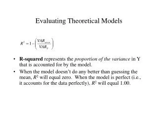
Evaluating The Validity of Models. In this class, we have focused on simple models, such as those predicting the variation in a single variable (Y). We want to know how good of a job the model does at accounting for the data. Assessing Model Fit.

E N D
Evaluating The Validity of Models • In this class, we have focused on simple models, such as those predicting the variation in a single variable (Y). • We want to know how good of a job the model does at accounting for the data.
Assessing Model Fit • If our model does a good job at accounting for Y, then the predicted Y values should be very close to the Y values we observe • (This notion of observed – expected will continue to reappear in the weeks to follow) • Note: We already have a way of quantifying this concept. We used it when trying to estimate the least-squares values of a and b in our linear model.
Assessing Model Fit • The average squared error, where “error” is defined as the difference between the observed and predicted values of the model • Recall that this quantity is a variance (average squared deviations from something = variance of something) • Thus, the error variance gives us an index of how “good” our model is in accounting for the data. • When the error variance is small, the model is doing well. When error variance is large, the model isn’t doing too well.
Large and Small • What exactly do we mean by “large” and “small” in this context? By “small,” the meaning should clear: A perfect model will have an error variance of exactly zero. • But, how large does the error variance have to be before we say the model is doing a poor job?
Quantifying large and small errors • Notice that this problem is similar to the one we confronted when considering the limitations of interpreting the magnitude of a covariance (which is, after all, a variance). • When the covariance between two variables is 0, we know how to interpret it. But we don’t know how to interpret a non-zero covariance very easily, and we need to interpret. • We need to interpret covariances relative to the maximum value they can take.
How big can the error variance get? • Similar situation: • How large would the error variance be if we were to make the best possible guesses about Y while ignoring our information about X? • Let’s explore the question at an intuitive level:
Guessing people’s scores on Y • Imagine that we are trying to guess peoples’ values of Y and that we have no information about their X values. • What would our best guess be? What would the intercept term be in this equation?
The mean as a best guess • If we are forced to guess, our best guess for each person is the mean of Y. • Why? The mean of Y can be conceptualized as a least-squares statistic, in the same sense that we have discussed a and b as being least-squares estimates. • Recall that the mean is defined as the balancing point for a set of scores, the point at which the sum of the deviations above that point are balanced by the sum of the deviations below that point.
The mean as a best guess • Mathematically, we defined the problem in the following way (weeks ago): (Y - M) = 0 • We could have also defined it as a least-squares estimation problem, one in which we are trying to find a value, M, that makes the following quantity as small as possible: (Y - M)2
The mean as a best guess • When we do this, we find that the value of M given by our trusty equation for the mean is the one that minimizes the function (Y - M)2 • (The guesses for M here are 1, 2, 3, 4, & 5. When M = 3, we have a minimum.)
The mean as a best guess • (Y - M)2 or • Notice that the quantity we are trying to minimize is a variance, specifically, the variance of Y. • In other words, when we use the classic equation for calculating M, we are finding a value, M, that makes the variance of Y as small as possible. If we had used any other value for M, our variance would be larger.
Why does all this matter? • If we want to predict peoples’ scores on Y in the absence of any information about X, we essentially want to pick a value that will minimize the squared differences between our guess and the actual values of Y (i.e., we want to minimize the error variance). • If we use the mean of Y as our best guess for each value of Y, we will be using the only value that makes the errors as small as possible. There is no other value we could use that would minimize these errors. Why? Because the mean of a variable is a least-squares statistic: It minimizes the variance.
Interim Summary • In the absence of information about X, we want to predict the Y scores as best as we can (i.e., we want to minimize the squared differences between the predicted and observed values) • The mean is a least-squares statistic. It minimizes the difference between “predicted” values and actual data. • The mean of Y is the best prediction we can make about the scores of Y in the absence of additional information.
Maximum possible error without knowing X • Now, let’s return to the question of finding the “maximum possible” error. • It follows from the previous points that • the “worst” we can do in predicting Y is getting an error variance that is as large as the actual variance of Y • When this happens, we are doing no better with our model than we would be doing if we were ignoring X and simply predicting Y on the basis of the mean of Y. • Thus, we can evaluate the quality of the model by comparing the error variance for the model with the variance of Y.
Maximum possible error • We can use these ideas to derive a quantitative index of model fit: how well the model does in accounting for the data proportion of variance in Y that is unexplained by the model proportion of variance in Y that is explained by the model
R-squared • This later quantity is often called R-squared, and represents the proportion of the variance in Y that is accounted for by the model • When the model doesn’t do any better than guessing the mean, R2 will equal zero. When the model is perfect (i.e., it accounts for the data perfectly), R2 will equal 1.00.
Neat fact • When dealing with a simple linear model with one X, R2 is equal to the correlation of X and Y, squared. • Why? Keep in mind that R2 is in a standardized metric in virtue of having divided the error variance by the variance of Y. Previously, when working with standardized scores in simple linear regression equations, we found that the parameter b is equal to r. Since b is estimated via least-squares techniques, it is directly related to R2.
Why is R2 useful? • R2 is useful because it is a standard metric for interpreting model fit. • It doesn’t matter how large the variance of Y is because everything is evaluated relative to the variance of Y • Set end-points: 1 is perfect and 0 is as bad as a model can be.