Exploring Linear Subspaces in High-Dimensional Image Variation and PCA
This document delves into linear subspaces and their applications in understanding variations in high-dimensional image data. Each image is represented as a point in a multidimensional space, where pixels serve as dimensions. The text discusses how principal component analysis (PCA) can approximate these images through lower-dimensional linear subspaces, minimizing distance from images to subspace. Additionally, concepts of removing translation and representation completeness are highlighted, providing insights into the geometric properties of image data.

Exploring Linear Subspaces in High-Dimensional Image Variation and PCA
E N D
Presentation Transcript
No Invariants, so Capture Variation • Each image = a pt. in a high-dimensional space. • Image: Each pixel a dimension. • Point set: Each coordinate of each pt. A dimension. • Simplest rep. of variation is linear. • Basis (eigen) images: x1…xk • Each image, x = a1x1 + … + akxk • Useful if k << n.
When is this accurate? • Approximately right when: • Variation approximately linear. Always true for small variation. • Some variations big, some small, can discard small. • Exactly right sometimes. • Point features with scaled-orthographic projection. • Convex, Lambertian objects and distant lights.
Principal Components Analysis (PCA) • All-purpose linear approximation. • Given images (as vectors) • Finds low-dimensional linear subspace that best approximates them. • Eg., minimizes distance from images to subspace.
Derivation on whiteboard • This is all taken from Duda, Hart and Stork Pattern Classification pp. 114-117. Excerpt in library.
SVD • Scatter matrix can be big, so computation non-trivial. • Stack data into matrix X, each row an image. SVD gives X = UDVT • D is diagonal with non-increasing values. • U and V have orthonormal rows. • VT(:,1:k) gives first k principal components. • matlab
Linear Combinations I S P Immediately apparent that u and v coordinates lie in a 4D linear subspace
We Can Remove Translation (1) • This is trivial, because we can pick a simple origin. • World origin is arbitrary. • Example: We can assume first point is at origin. • Rotation then doesn’t effect that point. • All its motion is translation. • Better to pick center of mass as origin. • Average of all points. • This also averages all noise.
Remove Translation (2) Notice this is just the first step of PCA.
Rank Theorem has rank 3. This means there are 3 vectors such that every row of is a linear combination of these vectors. These vectors are the rows of P. P S So, given any object, u and v coordinates of any image of it lie in a 3-dimensional linear subspace.
Lower-Dimensional Subspace • (a4,b4) = affine invariant coordinates of point 4 relative to first three. • Represent image: (a4,b4, a5,b5,…an,bn) • This representation is complete. • The a or b coordinates of all images of an object occupy a 1D linear subspace.
Representation is Complete • 3D-2D affine transformation is projection in some direction + 2D-2D affine transformation. • 2D-2D affine maps first three image points anywhere. So they’re irrelevant to a complete representation. • Once we use only affine coordinates, 2D-2D affine transformation no longer matters.
Summary • Projection can be linearized. • So images produced under projection can be linear and low-dimensional. • Are these results relevant to surfaces of real 3D objects projected to 2D? • Maybe to features; probably not to intensity images. • Why would images of a class of objects be low-dimensional?