Download
1 / 26
340 likes | 548 Views
S. S. D 1. A 1. D 2. A 2. A 3. D 3. Introduction to Wavelet. Bhushan D Patil PhD Research Scholar Department of Electrical Engineering Indian Institute of Technology, Bombay Powai, Mumbai. 400076. Outline of Talk. Overview Historical Development

E N D
S S D1 A1 D2 A2 A3 D3 Introduction to Wavelet Bhushan D Patil PhD Research Scholar Department of Electrical Engineering Indian Institute of Technology, Bombay Powai, Mumbai. 400076
Outline of Talk • Overview • Historical Development • Time vs Frequency Domain Analysis • Fourier Analysis • Fourier vs Wavelet Transforms • Wavelet Analysis • Typical Applications • References
OVERVIEW • Wavelet • A small wave • Wavelet Transforms • Convert a signal into a series of wavelets • Provide a way for analyzing waveforms, bounded in both frequency and duration • Allow signals to be stored more efficiently than by Fourier transform • Be able to better approximate real-world signals • Well-suited for approximating data with sharp discontinuities • “The Forest & the Trees” • Notice gross features with a large "window“ • Notice small features with a small
Historical Development • Pre-1930 • Joseph Fourier (1807) with his theories of frequency analysis • The 1930s • Using scale-varying basis functions; computing the energy of a function • 1960-1980 • Guido Weiss and Ronald R. Coifman; Grossman and Morlet • Post-1980 • Stephane Mallat; Y. Meyer; Ingrid Daubechies; wavelet applications today
Mathematical Transformation • Why • To obtain a further information from the signal that is not readily available in the raw signal. • Raw Signal • Normally the time-domain signal • Processed Signal • A signal that has been "transformed" by any of the available mathematical transformations • Fourier Transformation • The most popular transformation
FREQUENCY ANALYSIS • Frequency Spectrum • Be basically the frequency components (spectral components) of that signal • Show what frequencies exists in the signal • Fourier Transform (FT) • One way to find the frequency content • Tells how much of each frequency exists in a signal
STATIONARITY OF SIGNAL • Stationary Signal • Signals with frequency content unchanged in time • All frequency components exist at all times • Non-stationary Signal • Frequency changes in time • One example: the “Chirp Signal”
2 Hz + 10 Hz + 20Hz Magnitude Magnitude Stationary Time Frequency (Hz) 0.0-0.4: 2 Hz + 0.4-0.7: 10 Hz + 0.7-1.0: 20Hz Magnitude Magnitude Non-Stationary Time Frequency (Hz) STATIONARITY OF SIGNAL
Different in Time Domain Magnitude Magnitude Magnitude Magnitude Time Frequency (Hz) Time Frequency (Hz) CHIRP SIGNALS Frequency: 2 Hz to 20 Hz Frequency: 20 Hz to 2 Hz Same in Frequency Domain At what time the frequency components occur? FT can not tell!
NOTHING MORE, NOTHING LESS • FT Only Gives what Frequency Components Exist in the Signal • The Time and Frequency Information can not be Seen at the Same Time • Time-frequency Representation of the Signal is Needed Most of Transportation Signals are Non-stationary. (We need to know whether and also whenan incident was happened.) ONE EARLIER SOLUTION: SHORT-TIME FOURIERTRANSFORM(STFT)
SFORT TIME FOURIER TRANSFORM (STFT) • Dennis Gabor (1946) Used STFT • To analyze only a small section of the signal at a time -- a technique called Windowingthe Signal. • The Segment of Signal is Assumed Stationary • A 3D transform A function of time and frequency
DRAWBACKS OF STFT • Unchanged Window • Dilemma of Resolution • Narrow window -> poor frequency resolution • Wide window -> poor time resolution • Heisenberg Uncertainty Principle • Cannot know what frequency exists at what time intervals Via Narrow Window Via Wide Window
MULTIRESOLUTION ANALYSIS (MRA) • Wavelet Transform • An alternative approach to the short time Fourier transform to overcome the resolution problem • Similar to STFT: signal is multiplied with a function • Multiresolution Analysis • Analyze the signal at different frequencies with different resolutions • Good time resolution and poor frequency resolution at high frequencies • Good frequency resolution and poor time resolution at low frequencies • More suitable for short duration of higher frequency; and longer duration of lower frequency components
PRINCIPLES OF WAELET TRANSFORM • Split Up the Signal into a Bunch of Signals • Representing the Same Signal, but all Corresponding to Different Frequency Bands • Only Providing What Frequency Bands Exists at What Time Intervals
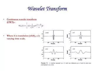
Translation (The location of the window) Scale Mother Wavelet DEFINITION OF CONTINUOUS WAVELET TRANSFORM • Wavelet • Small wave • Means the window function is of finite length • Mother Wavelet • A prototype for generating the other window functions • All the used windows are its dilated or compressed and shifted versions
SCALE • Scale • S>1: dilate the signal • S<1: compress the signal • Low Frequency -> High Scale -> Non-detailed Global View of Signal -> Span Entire Signal • High Frequency -> Low Scale -> Detailed View Last in Short Time • Only Limited Interval of Scales is Necessary
COMPUTATION OF CWT Step 1: The wavelet is placed at the beginning of the signal, and set s=1 (the most compressed wavelet); Step 2: The wavelet function at scale “1” is multiplied by the signal, and integrated over all times; then multiplied by ; Step 3: Shift the wavelet to t= , and get the transform value at t= and s=1; Step 4: Repeat the procedure until the wavelet reaches the end of the signal; Step 5: Scale s is increased by a sufficiently small value, the above procedure is repeated for all s; Step 6: Each computation for a given s fills the single row of the time-scale plane; Step 7: CWT is obtained if all s are calculated.
Better time resolution; Poor frequency resolution Frequency Better frequency resolution; Poor time resolution Time • Each box represents a equal portion • Resolution in STFT is selected once for entire analysis RESOLUTION OF TIME & FREQUENCY
From http://www.cerm.unifi.it/EUcourse2001/Gunther_lecturenotes.pdf, p.10 COMPARSION OF TRANSFORMATIONS
DISCRETIZATION OF CWT • It is Necessary to Sample the Time-Frequency (scale) Plane. • At High Scale s (Lower Frequency f ), the Sampling Rate N can be Decreased. • The Scale Parameter s is Normally Discretized on a Logarithmic Grid. • The most Common Value is 2. • The Discretized CWT is not a True Discrete Transform • Discrete Wavelet Transform (DWT) • Provides sufficient information both for analysis and synthesis • Reduce the computation time sufficiently • Easier to implement • Analyze the signal at different frequency bands with different resolutions • Decompose the signal into a coarse approximation and detail information
Multi Resolution Analysis • Analyzing a signal both in time domain and frequency domain is needed many a times • But resolutions in both domains is limited by Heisenberg uncertainty principle • Analysis (MRA) overcomes this , how? • Gives good time resolution and poor frequency resolution at high frequencies and good frequency resolution and poor time resolution at low frequencies • This helps as most natural signals have low frequency content spread over long duration and high frequency content for short durations
0-1000 Hz 256 Filter 1 X[n]512 D1: 500-1000 Hz 256 Filter 2 S S D2: 250-500 Hz 128 A1 D1 A1 128 Filter 3 D3: 125-250 Hz 64 D2 A2 A2 A3 D3 A3: 0-125 Hz 64 SUBBABD CODING ALGORITHM • Halves the Time Resolution • Only half number of samples resulted • Doubles the Frequency Resolution • The spanned frequency band halved
RECONSTRUCTION • What • How those components can be assembled back into the original signal without loss of information? • A Process After decomposition or analysis. • Also called synthesis • How • Reconstruct the signal from the wavelet coefficients • Where wavelet analysis involves filtering and down sampling, the wavelet reconstruction process consists of up sampling and filtering
WAVELET APPLICATIONS • Typical Application Fields • Astronomy, acoustics, nuclear engineering, sub-band coding, signal and image processing, neurophysiology, music, magnetic resonance imaging, speech discrimination, optics, fractals, turbulence, earthquake-prediction, radar, human vision, and pure mathematics applications • Sample Applications • Identifying pure frequencies • De-noising signals • Detecting discontinuities and breakdown points • Detecting self-similarity • Compressing images
REFERENCES • Mathworks, Inc. Matlab Toolbox http://www.mathworks.com/access/helpdesk/help/toolbox/wavelet/wavelet.html • Robi Polikar, The Wavelet Tutorial, http://users.rowan.edu/~polikar/WAVELETS/WTpart1.html • Robi Polikar, Multiresolution Wavelet Analysis of Event Related Potentials for the Detection of Alzheimer's Disease, Iowa State University, 06/06/1995 • Amara Graps, An Introduction to Wavelets, IEEE Computational Sciences and Engineering, Vol. 2, No 2, Summer 1995, pp 50-61. • Resonance Publications, Inc. Wavelets. http://www.resonancepub.com/wavelets.htm • R. Crandall, Projects in Scientific Computation, Springer-Verlag, New York, 1994, pp. 197-198, 211-212. • Y. Meyer, Wavelets: Algorithms and Applications, Society for Industrial and Applied Mathematics, Philadelphia, 1993, pp. 13-31, 101-105. • G. Kaiser, A Friendly Guide to Wavelets, Birkhauser, Boston, 1994, pp. 44-45. • W. Press et al., Numerical Recipes in Fortran, Cambridge University Press, New York, 1992, pp. 498-499, 584-602. • M. Vetterli and C. Herley, "Wavelets and Filter Banks: Theory and Design," IEEE Transactions on Signal Processing, Vol. 40, 1992, pp. 2207-2232. • I. Daubechies, "Orthonormal Bases of Compactly Supported Wavelets," Comm. Pure Appl. Math., Vol 41, 1988, pp. 906-966. • V. Wickerhauser, Adapted Wavelet Analysis from Theory to Software, AK Peters, Boston, 1994, pp. 213-214, 237, 273-274, 387. • M.A. Cody, "The Wavelet Packet Transform," Dr. Dobb's Journal, Vol 19, Apr. 1994, pp. 44-46, 50-54. • J. Bradley, C. Brislawn, and T. Hopper, "The FBI Wavelet/Scalar Quantization Standard for Gray-scale Fingerprint Image Compression," Tech. Report LA-UR-93-1659, Los Alamos Nat'l Lab, Los Alamos, N.M. 1993. • D. Donoho, "Nonlinear Wavelet Methods for Recovery of Signals, Densities, and Spectra from Indirect and Noisy Data," Different Perspectives on Wavelets, Proceeding of Symposia in Applied Mathematics, Vol 47, I. Daubechies ed. Amer. Math. Soc., Providence, R.I., 1993, pp. 173-205. • B. Vidakovic and P. Muller, "Wavelets for Kids," 1994, unpublished. Part One, and Part Two.