Download
1 / 23
230 likes | 249 Views
Learn how to estimate and test overall or typical effects using the fixed-effects and random-effects models in meta-analysis.

E N D
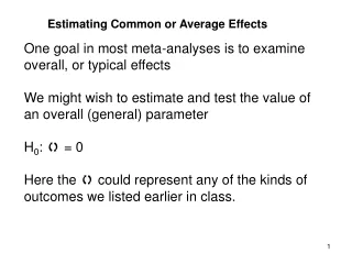
Estimating Common or Average Effects One goal in most meta-analyses is to examine overall, or typical effects We might wish to estimate and test the value of an overall (general) parameter H0: = 0 Here the could represent any of the kinds of outcomes we listed earlier in class.
Estimating Common or Average Effects Under the random-effects model, we can test H0: = 0 e.g., H0: = 0 The average of The average of the i values the population is zero correlations is zero Formulas for estimates of these parameters will follow.
Estimating Common or Average Effects We saw above that the fixed-effects mean for the teacher expectancy data was Also our SPSS output showed a random-effects mean for the TE data of Why are they different?
The FE mean is pulled towards the large studies with low effects like 6, 7, and 18. RE FE The RE mean is just a bit higher.
Estimating Common Effects For the fixed-effects model, and to get Q, we compute an effect that we will assume is common to all studies. Our book calls this M but I prefer to call it . We use a weighted mean – weighting each data point by the inverse of its variance (i.e., wi = 1/V(Ti) = 1/Vi ):
Estimating Common Effects Since we need the FE mean for the test of homogeneity we can get it from SPSS code or from pull-down analyses or from R code. However we must decide whether to report it or not.
Estimating Average Effects For the random-effects model, we compute an average of the effects that we believe truly vary across studies. The model for the effect size was Ti = θi + ei with variance V(Ti) = Vi* = s2θ + Vi . We use an estimate to get new V* variances and weights that incorporate both parts of the variation in the effects Ti.
These RE CIs are made using the new RE variances Vi* RE FE The RE CIs are more equal in width and studies have very similar influence on the mean.
Estimating Average Effects For RE we weight each data point by the new RE weight -- the inverse of its random-effects variance: w*i = 1/[Vi + ] Thus to get the RE mean we compute
The FE variances (V) range from about .01 to .14. This is fairly typical. Large n go with small V. We added .08 to each V value to get the RE variance V*.
The ratio of the largest weight to the smallest one is 16:1 for the FE weights (w) but it is only 2.5:1 for the RE weights (wstar). Large studies do not have as much relative influence under the RE model.
Estimating Common Effects We also need a variance (or standard error) for the mean. To compute the SE for the fixed effects case we use the inverse variances of the individual effects – or equivalently the weights. The variance of the fixed-effects mean is and the SE is the square root of the variance.
Estimating Common Effects The variance (or SE) for the random-effects mean is very similar to the FE variance and the SE is the square root of the variance. This variance will be larger than the FE variance because of the addition of to each Vi
Random-effects variancesHowever we have not seen how to estimate 2 We will consider two method-of-moments estimators. I call them SVAR and QVAR in our programs.SVAR is based on a “typical” sample variance of the T’s (like you learned in intro stats class) and QVAR is computed using Q thus it is weighted. These are not the “best” variance estimates but are easily obtained using SPSS.
Random-effects variances: SVARSVAR uses the sample variance of the T’s. In the random-effects model Ti = i + ei. Therefore V(Ti) = V(i) + V(ei) so V(Ti) - V(ei) = V(i)We then get the expected values of each part E[V(Ti)] – E[V(ei)] = E[V(i)] = 2 So our estimator is SVAR = ST2 -
Random-effects variances: QVARQVAR is computed using Q and some sums of the weights wi and squared weights wi2The amount by which Q exceeds its df (for the total Q, df=k-1) is the part due to “true” differences, not sampling error There is no good non-technical explanation of how the weights work here, but the formula is QVAR = ( Q ‑ (k-1) ) wi ‑ (wi2/ wi )
The SPSS output also gives the two values of QVAR and SVAR. Fixed-effects Homogeneity Test (Q) 35.8254 P-value for Homogeneity test (P) .0074 Birge's ratio, ratio of Q/(k-1) 1.9903 I-squared, ratio 100 [Q-(k-1)]/Q .4976 Variance Component based on Homogeneity Test (QVAR) .0259 Variance Component based on S2 and v-bar (SVAR) .0804 RE Lower Conf Limit for T_Dot (L_T_DOT) -.0410 Weighted random-effects average of effect size based on SVAR (T_DOT) .1143 RE Upper Conf Limit for T_Dot (U_T_DOT) .2696
Finally we return to slides 9 and 13, and add to the Vi values to get the RE mean and its SE. The new RE mean is larger and its SE is larger. The new SE is over twice the size of the FE standard error. Thus the random effects CI is also more than twice as wide.
In this case we decide that the mean effect size is not different from zero based on the CI. We can also test H0: = 0 using the RE mean and SE: Z = T.*/SE(T.*) = 0.11/0.079 = 1.329 We compare this sample Z to a critical Z value such as ZC = +1.96 for a two-tailed test at a = .05. This Z is not large enough to reject H0. On average the teacher expectancy effect is about a tenth of a standard deviation in the sample, but there is essentially no true difference.
However some studies show effects much larger than 0.11. Now we can separately interpret . Our best estimate of the mean of the population effects is 0.11 and their estimated variance is 0.08 (SD = .28). This is NOT the same as the SE of the mean effect, which was 0.079 on the previous slides. The values of SVAR and QVAR tell us how spread out the population of effects seems to be.
We can use the estimate of to draw a picture of the population of effects. The estimated variance of the population effects is 0.08 (SD = .28). We assume a normal shape for the population and center it on the RE mean. If the effects were normally distributed – the distribution of TRUE effects would look like this. 95% of the dis would be between about -0.44 and 0.66.
The previous slide contains excel code that allows you to make a graph of your own data. You need to double click the plot, then you will see a spreadsheet. Go to the tab labeled normal. Enter a new mean for the population (where you see 0.11) and a new SD (replace .283), then go back to the Chart tab.
Mixed Effects Models If each population effect differs, and Ti = i + ei we may want to model or explain the variation in the population effects. For example we may have i = b0 + b1X1i + u’i Substituting, we have Ti =b0 + b1X1i + u’i + ei Observed Effect predicted + Unexplained between- + Sampling effect from X value studies variation error