Download
1 / 19
210 likes | 393 Views
Linear Regression t-Tests. Cardiovascular fitness among skiers. Cardiovascular fitness is measured by the time required to run to exhaustion on a treadmill. In the following study, cardiovascular fitness is compared to performance in a 20-km ski race.

E N D
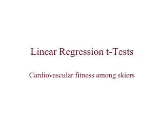
Linear Regression t-Tests Cardiovascular fitness among skiers
Cardiovascular fitness is measured by the time required to run to exhaustion on a treadmill. In the following study, cardiovascular fitness is compared to performance in a 20-km ski race. The following data are for biathletes, as reported in an article on sports physiology: x = treadmill time (minutes) y = 20-km ski time (minutes) “Physiological Characteristics and Performance of Top U.S. Biathletes” (Medicine and Science in Sports and Exercise(1995):1302-1310.
When we encounter data in ordered pairs we usually examine the data first by making a scatterplot. First, we will enter the data into lists on the calculator. Now setting up the scatterplot: The scatterplot suggests a negative linear relationship between treadmill time and ski race time. Note that while my graphs do not have axes labeled, this is due to technical constraints, and when you write your answers on paper you should always label the axes and show the scale.
We perform linear regression to obtain the equation of the best-fit line. On the TI-83 press <STAT> <CALC> <8:LinReg(a+bx)> Recall that L1 and L2 are the default lists so I don’t have to specify them, but do need to specify Y1 in order to store the equation: Press <VARS> <Y-VARS> <1:Function> <1:Y1> Press <ENTER>.
The linear model shows that for every minute increase in treadmill time there is a decrease of 2.3335 minutes (on average) in ski race time. When the treadmill time is zero, the ski race time is expected to be 88.795 minutes. Now graphing the line we see that the model looks good. Recall that whenever we perform linear regression we must confirm our results by making a residual plot.
To make a scatterplot of the residuals, set up the scatterplot, as usual. To enter the residuals in the Ylist, press <2nd> <LIST> then scroll to <RESID> . Press <ZOOM> <STAT> to see the image. Here we see that the residuals are fairly randomly scattered. This patternless residual plot allows us to confirm our linear model for the data.
A new concern for us in this new test is that our residuals need to be normally distributed. This meets a requirement that the response variable varies normally. We have not seen this assumption before. We have in the past needed to establish that data is derived from a normal distribution. We will follow the same approach here.
We make a normal probability plot to check this. The normal probability plot shows a linear pattern. This is consistent with the residuals having a normal distribution. Another piece of information we need for the linear regression t-test deals with an assumption that the standard deviation is the same far all values of x. To check this we reexamine the residual plot.
If the data are scattered to about the same extent as we move from left to right, we can say that the equal variance assumption is met. Some people call this visual inspection the Does the plot thicken? condition. That is, do the residuals get closer together in part of the graph? In our example the variance seems the same throughout. We really just have one more assumption, and that is that the individual ordered pairs are independent of one another. In practice this is difficult to truly satisfy, and we often move forward without fully knowing that the data is independent.
The best we can do is carefully examine the data and the residuals, looking for patterns that we might have overlooked. If data is collected over time, we might want to graph it as a function of time to see if there has been a general trend that would represent a violation of the independence assumption.
Now we look more towards the test. If we make repeated samples of data from a population and fit each sample with linear regression, we will likely get different equations each time. We understand that, due to sampling variability, our estimates of aand bin the equation are just that, estimates. Since we calculate them on samples they are statistics. They estimate values that are true for the population. Ultimately, we seek the true regression line, and write it with Greek letters for the parameters αand β.
The null hypothesis is always The alternate hypothesis is always The true regression line is Our significance test will attempt to determine whether β is zero. If the slope is zero then the explanatory variable is useless as a predictor of the response variable.
For us to be able to judge whether the variability we see is explainable by chance alone, we must have an idea of how much variability there is in this system. We calculate the standard error about the line. We use s to estimate σin the regression model.
We have degrees of freedom in this test because it is a t-test. We will have n-2 degrees of freedom in these tests, where n is the number of data points. We need one further concept, and that is of standard error of the regression slope SEb.. We are now ready to define our test statistic:
Step 1: Step 2: Let’s give a quick example of how you should write this as a 7-step write-up. This scatterplot shows a negative linear relationship between treadmill time and ski-race time. where x is treadmill time and y is ski time
This residual plot is patternless, which is consistent with our linear model. Further examination of this residual plot shows that the standard deviation is the same throughout. A linear form of the normal probability plot shows that the residuals appear to fit a normal model.
Step 3: df = 9. Our data appear to be independent since treadmill measures would be made independently of the ski race. This was found by running the linear regression t-test on the calculator . To do this press <STAT> <TESTS> <F:LinRegTTest> <ENTER>. Set the values, as shown.
Step 5: Step 7: Step 4: Step 6: The test statistic is too extreme to see the shading on this graph. Reject H0, a value this extreme may occur by chance alone less than 1% of the time. We have evidence that cardiovascular fitness, as measured by a treadmill test, does correspond to reduced race time on 20-km ski race.