Multiple Alignment
Multiple Alignment. Anders Gorm Pedersen Molecular Evolution Group Center for Biological Sequence Analysis gorm@cbs.dtu.dk. Refresher: pairwise alignments. 43.2% identity; Global alignment score: 374 10 20 30 40 50


Multiple Alignment
E N D
Presentation Transcript
Multiple Alignment Anders Gorm Pedersen Molecular Evolution Group Center for Biological Sequence Analysis gorm@cbs.dtu.dk
Refresher: pairwise alignments 43.2% identity; Global alignment score: 374 10 20 30 40 50 alpha V-LSPADKTNVKAAWGKVGAHAGEYGAEALERMFLSFPTTKTYFPHF-DLS-----HGSA : :.: .:. : : :::: .. : :.::: :... .: :. .: : ::: :. beta VHLTPEEKSAVTALWGKV--NVDEVGGEALGRLLVVYPWTQRFFESFGDLSTPDAVMGNP 10 20 30 40 50 60 70 80 90 100 110 alpha QVKGHGKKVADALTNAVAHVDDMPNALSALSDLHAHKLRVDPVNFKLLSHCLLVTLAAHL .::.::::: :.....::.:.. .....::.:: ::.::: ::.::.. :. .:: :. beta KVKAHGKKVLGAFSDGLAHLDNLKGTFATLSELHCDKLHVDPENFRLLGNVLVCVLAHHF 60 70 80 90 100 110 120 130 140 alpha PAEFTPAVHASLDKFLASVSTVLTSKYR :::: :.:. .: .:.:...:. ::. beta GKEFTPPVQAAYQKVVAGVANALAHKYH 120 130 140
Refresher: pairwise alignments • Alignment score is calculated from substitution matrix • Identities on diagonal have high scores • Similar amino acids have high scores • Dissimilar amino acids have low (negative) scores • Gaps penalized by gap-opening + gap elongation A 5 R -2 7 N -1 -1 7 D -2 -2 2 8 C -1 -4 -2 -4 13 Q -1 1 0 0 -3 7 E -1 0 0 2 -3 2 6 G 0 -3 0 -1 -3 -2 -3 8 . . . A R N D C Q E G ... K L A A S V I L S D A L K L A A - - - - S D A L -10 + 3 x (-1)=-13
Refresher: pairwise alignments The number of possible pairwise alignments increases explosively with the length of the sequences: Two protein sequences of length 100 amino acids can be aligned in approximately 1060 different ways 1060 bottles of beer would fill up our entire galaxy
Refresher: pairwise alignments • Solution: dynamic programming • Essentially: the best path through any grid point in the alignment matrix must originate from one of three previous points • Far fewer computations • Best alignment guaranteed to be found T C G C A T C C A x
Refresher: pairwise alignments • Most used substitution matrices are themselves derived empirically from simple multiple alignments A/A 2.15% A/C 0.03% A/D 0.07% ... Calculate substitution frequencies Multiple alignment Convert to scores Freq(A/C),observed Freq(A/C),expected Score(A/C) = log
Multiple alignments: what use are they? • Starting point for studies of molecular evolution
Multiple alignments: what use are they? • Characterization of protein families: • Identification of conserved (functionally important) sequence regions • Prediction of structural features (disulfide bonds, amphipathic alpha-helices, surface loops, etc.)
Scoring a multiple alignment:the “sum of pairs” score AA: 4, AS: 1, AT:0 AS: 1, AT: 0 ST: 1 Score: 4+1+0+1+0+1 = 7 ...A... ...A... ...S... ...T... One column from alignment • In theory, it is possible to define an alignment score for multiple alignments (there are many alternative scoring systems)
Multiple alignment: dynamic programming is only feasible for very small data sets • In theory, optimal multiple alignment can be found by dynamic programming using a matrix with more dimensions (one dimension per sequence) • BUT even with dynamic programming finding the optimal alignment very quickly becomes impossible due to the astronomical number of computations • Full dynamic programming only possible for up to about 4-5 protein sequences of average length • Even with heuristics, not feasible for more than 7-8 protein sequences • Never used in practice Dynamic programming matrix for 3 sequences For 3 sequences, optimal path must come from one of 7 previous points
Multiple alignment: an approximate solution • Progressive alignment (ClustalX and other programs): • Perform all pairwise alignments; keep track of sequence similarities between all pairs of sequences (construct “distance matrix”) • Align the most similar pair of sequences • Progressively add sequences to the (constantly growing) multiple alignment in order of decreasing similarity.
Progressive alignment: details Perform all pairwise alignments, note pairwise distances (construct “distance matrix”) 2) Construct pseudo-phylogenetic tree from pairwise distances S1 S2 S3 S4 S1 S2 3 S3 1 3 S4 3 2 3 S1 S2 S3 6 pairwise alignments S4 S1 S2 S3 S4 S1 S2 3 S3 1 3 S4 3 2 3 S1 S3 S4 S2 “Guide tree”
Progressive alignment: details • Use tree as guide for multiple alignment: • Align most similar pair of sequences using dynamic programming • Align next most similar pair • Align alignments using dynamic programming - preserve gaps S1 S3 S1 S3 S4 S2 S2 S4 S1 S3 S2 S4 New gap to optimize alignment of (S2,S4) with (S1,S3)
Aligning profiles S1 S3 Aligning alignments: each alignment treated as a single sequence (a profile) + S2 S4 Full dynamic programming on two profiles S1 S3 S2 S4 New gap to optimize alignment of (S2,S4) with (S1,S3)
Scoring profile alignments Compare each residue in one profile to all residues in second profile. Score is average of all comparisons. ...A... ...S... AS: 1, AT:0 SS: 4, ST:1 Score: 1+0+4+1 = 1.5 + ...S... ...T... 4 One column from alignment
Additional ClustalX heuristics • Sequence weighting: • scores from similar groups of sequences are down-weighted • Variable substitution matrices: • during alignment ClustalX uses different substitution matrices depending on how similar the sequences/profiles are • Variable gap penalties: • gap penalties depend on substitution matrix • gap penalties depend on similarity of sequences • reduced gap penalties at existing gaps • increased gap penalties CLOSE to existing gaps • reduced gap penalties in hydrophilic stretches (presumed surface loop) • residue-specific gap penalties • and more...
Other multiple alignment programs ClustalW / ClustalX pileup multalign multal saga hmmt DIALIGN SBpima MLpima T-Coffee ...
Other multiple alignment programs ClustalW / ClustalX pileup multalign multal saga hmmt DIALIGN SBpima MLpima T-Coffee ...
Global methods (e.g., ClustalX) get into trouble when data is not globally related!!!
Global methods (e.g., ClustalX) get into trouble when data is not globally related!!! Clustalx
Global methods (e.g., ClustalX) get into trouble when data is not globally related!!! Clustalx • Possible solutions: • Cut out conserved regions of interest and THEN align them • Use method that deals with local similarity (e.g. DIALIGN)
Brief Introduction to the Theory of Evolution Anders Gorm Pedersen Molecular Evolution Group Center for Biological Sequence Analysis gorm@cbs.dtu.dk
Classification: Linnaeus Carl Linnaeus 1707-1778
Classification: Linnaeus • Hierarchical system • Kingdom (Rige) • Phylum (Række) • Class (Klasse) • Order (Orden) • Family (Familie) • Genus (Slægt) • Species (Art)
Classification depicted as a tree Species Genus Family Order Class
Theory of evolution Charles Darwin 1809-1882
Phylogenetic basis of systematics • Linnaeus: Ordering principle is God. • Darwin: Ordering principle is shared descent from common ancestors. • Today, systematics is explicitly based on phylogeny.
Darwin’s four postulates • More young are produced each generation than can survive to reproduce. • Individuals in a population vary in their characteristics. • Some differences among individuals are based on genetic differences. • Individuals with favorable characteristics have higher rates of survival and reproduction. • Evolution by means of natural selection • Presence of ”design-like” features in organisms: quite often features are there “for a reason”
Theory of evolution as the basis of biological understanding ”Nothing in biology makes sense, except in the light of evolution. Without that light it becomes a pile of sundry facts - some of them interesting or curious but making no meaningful picture as a whole” T. Dobzhansky
Phylogenetic Reconstruction:Distance Matrix Methods Anders Gorm Pedersen Molecular Evolution Group Center for Biological Sequence Analysis Technical University of Denmark gorm@cbs.dtu.dk
Trees: representations Three different representations of the same tree
Trees: rooted vs. unrooted • A rooted tree has a single node (the root) that represents a point in time that is earlier than any other node in the tree. • A rooted tree has directionality (nodes can be ordered in terms of “earlier” or “later”). • In the rooted tree, distance between two nodes is represented along the time-axis only (the second axis just helps spread out the leafs) Early Late
Trees: rooted vs. unrooted • A rooted tree has a single node (the root) that represents a point in time that is earlier than any other node in the tree. • A rooted tree has directionality (nodes can be ordered in terms of “earlier” or “later”). • In the rooted tree, distance between two nodes is represented along the time-axis only (the second axis just helps spread out the leafs) Early Late
Trees: rooted vs. unrooted • A rooted tree has a single node (the root) that represents a point in time that is earlier than any other node in the tree. • A rooted tree has directionality (nodes can be ordered in terms of “earlier” or “later”). • In the rooted tree, distance between two nodes is represented along the time-axis only (the second axis just helps spread out the leafs) Early Late
Trees: rooted vs. unrooted • In unrooted trees there is no directionality: we do not know if a node is earlier or later than another node • Distance along branches directly represents node distance
Trees: rooted vs. unrooted • In unrooted trees there is no directionality: we do not know if a node is earlier or later than another node • Distance along branches directly represents node distance
Data: molecular phylogeny • DNA sequences • genomic DNA • mitochondrial DNA • chloroplast DNA • Protein sequences • Restriction site polymorphisms • DNA/DNA hybridization • Immunological cross-reaction
Morphology vs. molecular data African white-backed vulture (old world vulture) Andean condor (new world vulture) New and old world vultures seem to be closely related based on morphology. Molecular data indicates that old world vultures are related to birds of prey (falcons, hawks, etc.) while new world vultures are more closely related to storks Similar features presumably the result of convergent evolution
Molecular data: single-celled organisms Molecular data useful for analyzing single-celled organisms (which have only few prominent morphological features).
Distance Matrix Methods • Construct multiple alignment of sequences • Construct table listing all pairwise differences (distance matrix) • Construct tree from pairwise distances Gorilla : ACGTCGTA Human : ACGTTCCT Chimpanzee: ACGTTTCG Ch 1 1 1 Hu 2 Go
Finding Optimal Branch Lengths S2 S1 a c b e d S3 S4 Distance along tree Observed distance D12 d12 = a + b + c D13 d13 = a + d D14 d14 = a + b + e D23 d23 = d + b + c D24 d24 = c + e D34 d34 = d + b + e Goal:
Optimal Branch Lengths: Least Squares • Fit between given tree and observed distances can be expressed as “sum of squared differences”: Q = (Dij - dij)2 • Find branch lengths that minimize Q - this is the optimal set of branch lengths for this tree. S2 S1 a c b e d S3 S4 Distance along tree j>i D12 d12 = a + b + c D13 d13 = a + d D14 d14 = a + b + e D23 d23 = d + b + c D24 d24 = c + e D34 d34 = d + b + e Goal:
Least Squares Optimality Criterion • Search through all (or many) tree topologies • For each investigated tree, find best branch lengths using least squares criterion • Among all investigated trees, the best tree is the one with the smallest sum of squared errors.