Download
1 / 32
320 likes | 386 Views
RAISHIN is a 3D GRMHD code utilizing high-resolution shock capturing schemes, special & general relativity, different coordinate systems, parallel computing, and various numerical accuracy schemes.

E N D
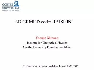
3D GRMHD code: RAISHIN Yosuke Mizuno Institute for Theoretical Physics Goethe University Frankfurt am Main BH Cam code-comparison workshop, January 20-21, 2015
Code General Information Mizuno et al. 2006a, 2011c, & progress • RAISHIN utilizes conservative, high-resolution shock capturing schemes (Godunov-type scheme) to solve the 3D ideal GRMHD equations (metric is static) • Program Language: Fortran 90 • Multi-dimension (1D, 2D, 3D) • Special & General relativity (static metric), three different code package • Different coordinates (RMHD: Cartesian, Cylindrical, Spherical and GRMHD: Boyer-Lindquist coordinates and Kerr-Schild coordinates) • Different schemes of numerical accuracy for numerical model (spatial reconstruction, approximate Riemann solver, constrained transport schemes, time advance, & inversion) • Using constant G-law, polytropic, and approximate Equation of State (Synge-type) • Uniform & non-uniform grid • Parallel computing (based on MPI)
Basic Equations (SRMHD) Conserved Form Flux Primitive variables Conserved variables Magnetic field 4-vector (Magnetic field measured in comoving frame)
Basic Equations (GRMHD) Metric Conserved Form a: lapse function, bi: shift vector Flux Conserved variables Primitive variables Source term Magnetic field 4-vector Energy-momentum tensor
Flow Chart for Calculation • Reconstruction • (Pn : cell-center to cell-surface) • 2. Calculation of Flux at cell-surface • 3. Integrate hyperbolic equations => Un+1 • 4. Convert from Un+1 to Pn+1 Primitive Variables: P Conserved Variables: U Flux: F Source: S Ui Fi-1/2 Fi+1/2 Pi-1 Pi+1 Pi Si
Reconstruction • Minmod & MCFlux-limiter (Piecewise linear Method) • 2nd order at smooth region • Convex ENO (Liu & Osher 1998) • 3rd order at smooth region • Piecewise Parabolic Method (Marti & Muller 1996) • 4th order at smooth region • Weighted ENO, WENO-Z, WENO-M (Jiang & Shu 1996; Borges et al. 2008) • 5th order at smooth region • Monotonicity Preserving (Suresh & Huynh 1997) • 5th order at smooth region • MPWENO5 (Balsara & Shu 2000) • Logarithmic 3rd order limiter (Cada & Torrilhon 2009) Cell-centered variables (Pi) → right and left side of Cell-interface variables(PLi+1/2, PRi+1/2) Piecewise linear interpolation PLi+1/2 PRi+1/2 Pni-1 Pni Pni+1
Approximate Riemann Solver • Calculate numerical flux at cell-inteface from reconstructed cell-interface variables based on Riemann problem • We use HLL approximate Riemann solver • Need only the maximum left- and right- going wave speeds (in MHD case, fast magnetosonic mode) lR, lL: fastest characteristic speed HLL flux lL t lR M Ui Fi-1/2 Fi+1/2 R L x Pi-1 Pi+1 Pi If lL >0 FHLL=FL lL < 0 < lR , FHLL=FM lR < 0 FHLL=FR
Approximate Riemann Solver • HLL Approximate Riemann solver: single state in Riemann fan • HLLC Approximate Riemann solver: two-state in Riemann fan (Mignone & Bodo 2006, Honkkila & Janhunen2007) (for SRMHD only) • HLLD Approximate Riemann solver: six-state in Riemann fan (Mignone et al. 2009) (for SRMHD only) • Roe-type full wave decomposition Riemann solver(Anton et al. 2010)
Wave speed • To calculate numerical flux at each cell-boundary via Riemann solver, we need to know wave speed in each directions lE=vi, entropy wave Alfven waves Magneto-acoustic waves are found from the quartic equation • Some simple estimation for fast magnetosonic wave • => Leismann et al. (2005), no numerical iteration
Constrained Transport Differential Equations • The evolution equation can keep divergence free magnetic field • If treat the induction equation as all other conservation laws, it can not maintain divergence free magnetic field • → We need spatial treatment for magnetic field evolution • Constrained transport scheme • Evans & Hawley’s Constrained Transport (need staggered mesh) • Toth’s constrained transport (flux-CT) (Toth 2000) for SRMHD & GRMHD • Fixed Flux-CT, Upwind Flux-CT (Gardiner & Stone 2005, 2007), for SRMHD only • Other method • Diffusive cleaning (GLM formulation) for RRMHD only
Time evolution System of Conservation Equations We use multistep TVD Runge-Kutta method for time advance of conservation equations (RK2: 2nd-order, RK3: 3rd-order in time) RK2, RK3: first step RK2: second step (a=2, b=1) RK3: second and third step (a=4, b=3)
Recovery step • The GRMHD code require a calculation of primitive variables from conservative variables. • The forward transformation (primitive → conserved) has a close-form solution, but the inverse transformation (conserved → primitive) requires the solution of a set of five nonlinear equations Method • Noble’s 2D method (Noble et al. 2005) • Mignone & McKinney’s method (Mignone & McKinney 2007)
General (Approximate) EoS Mignone & McKinney 2007 • In the theory of relativistic perfect single gases, specific enthalpy is a function of temperature alone (Synge 1957) Q: temperature p/r K2, K3: the order 2 and 3 of modified Bessel functions • Constant G-law EoS (ideal EoS) : • G: constant specific heat ratio • Taub’s fundamental inequality(Taub 1948) Q → 0, Geq → 5/3, Q → ∞, Geq → 4/3 Solid: Synge EoS Dotted: ideal + G=5/3 Dashed: ideal+ G=4/3 Dash-dotted: TM EoS • TM EoS (approximate Synge’s EoS) • (Mignone et al. 2005) c/sqrt(3)
Code Accuracy (L1 norm) 1D CP Alfven wave propagation test L1 norm errors of magnetic field vy shows almost 2nd order accuracy
Code Accuracy (grid number vs computer time) 1D shock-tube (Balsara Test 1) with 1 CPU calculated to t=0.4 tsim ∝ Nx2 Number of grid
Parallelization Accuracy 1D shock-tube (Balsara Test 1) in 3D Cartesian box, calculated to t=0.4 99% 98% 90% T(1) / T(N) Number of CPU
1D Relativistic MHD Shock-Tube Mizuno et al. 2006 Balsara Test1 (Balsara 2001) • The results show good agreement of the exact solution calculated by Giacommazo & Rezzolla (2006). • Minmod slope-limiter and CENO reconstructions are more diffusive than the MC slope-limiter and PPM reconstructions. • Although MC slope limiter and PPM reconstructions can resolve the discontinuities sharply, some small oscillations are seen at the discontinuities. FR SR SS FR CD Black: exact solution, Blue: MC-limiter, Light blue: minmod-limiter, Orange: CENO, red: PPM 400 computational zones
Advection of Magnetic Field Loop 2D No advection • Advection of a weak magnetic field loop in an uniform velocity field • 2D: (vx, vy)=(0.6,0.3) • 3D: (vx,vy,vz)=(0.3,0.3,0.6) • Periodic boundary in all direction • Run until return to initial position in advection case B2 Advection Volume-averaged magnetic energy density (2D) 3D B2 Nx=512 256 128 Advection No advection
1D Bondi Accretion 1D Bondi flow with radial B-field (b=1) G=4/3, rc=8rg r/rg Results follow initial Bondi flow structure ur vr r/rg r/rg
2D torus (Hydro) • 2D geometrically thick torus (Fishbone & Moncrief 1976) with no magnetic field. • a/M=0, Kerr-Schild coordinates r
Ideal / Resistive RMHD Eqs Ideal RMHD Resistive RMHD Solve 11 equations (8 in ideal MHD) Need a closure relation between J and E => Ohm’s law
Ohm’s law • Relativistic Ohm’s law (Blackman & Field 1993 etc.) isotropic diffusion in comoving frame (most simple one) Lorentz transformation in lab frame Relativistic Ohm’s law with istoropic diffusion • ideal MHD limit (conductivity: s => infinity) Charge current disappear in the Ohm’s law (degeneracy of equations, EM wave is decupled)
Numerical Integration Resistive RMHD Constraint Hyperbolic equations Solve Relativistic Resistive MHD equations by taking care of 1. stiff equations appeared in Ampere’s law 2. constraints ( no monopole, Gauss’s law) 3. Courant conditions (the largest characteristic wave speed is always light speed.) Source term Stiff term
Difficulty of RRMHD 1. Constraint should be satisfied bothconstraint numerically 2. Ampere’s law Equation becomes stiff at high conductivity
Constraints Approaching Divergence cleaning method (Dedner et al. 2002, Komissarov 2007) Introduce additional field F & Y (for numerical noise) advect & decay in time
Stiff Equation Komissarov (2007) Problem comes from difference between dynamical time scale and diffusive time scale => analytical solution Ampere’s law diffusion (stiff) term Operator splitting method Hyperbolic + source term Solve by HLL method Analytical solution source term (stiff part) Solve (ordinary differential) eqaution
Flow Chart for Calculation (RRMHD) Strang Splitting Method Step1: integrate diffusion term in half-time step Step2: integrate advection term in half-time step Un=(En+1/2, Bn) Step3: integrate advection term in full-time step Step4: integrate diffusion term in full-time step (En+1, Bn+1)=Un+1
1D Shock-Tube Test (Brio & Wu) • Aim: Check the effect of resistivity (conductivity) • Simple MHD version of Brio & Wu test • (rL, pL, ByL) = (1, 1, 0.5), (rR, pR, ByR)=(0.125, 0.1, -0.5) • Ideal EoS with G=2 Orange solid: s=0 Green dash-two-dotted: s=10 Red dash-dotted: s=102 Purple dashed: s=103 Blue dotted: s=105 Black solid: exact solution in ideal RMHD Smooth change from a wave-like solution (s=0) to ideal-MHD solution (s=105)
Relativistic Magnetic Reconnection • Assumption • Consider Pestchek-type magnetic reconnection • Initial condition • Harris-type model(anti-parallel magnetic field) • Anomalous resistivity for triggering magnetic reconnection (r<0.8) • Results • B-filed:typical X-type topology • Density:Plasmoid • Reconnection outflow: ~0.8c
Summary of RAISHIN code • RAISHIN utilizes conservative, high-resolution shock capturing schemes (Godunov-type scheme) to solve the 3D ideal GRMHD equations (metric is static) • Program Language: Fortran 90 • Multi-dimension (1D, 2D, 3D) • Special & General relativity (static metric), three different code package (SRMHD, GRMHD, RRMHD) • Different coordinates (SRMHD: Cartesian, Cylindrical, Spherical and GRMHD: Boyer-Lindquist coordinates and Kerr-Schild coordinates) • Different schemes is applied in each steps • Using constant G-law, polytropic, and approximate Equation of State (Synge-type) • Parallel computing (based on MPI)