Download
1 / 25
250 likes | 271 Views
Learn about heat budget components, short and long wave radiation, penetration of radiation, latent heat flux, and more in temperature models. Explore calculation options and solution principles for accurate temperature modeling. Gain insights from experiences with the PROBE-model.

E N D
2. Temperature models Huttula Lecture set 2
Heat balance components Heat budget is calculated as water balance. We need to know the components in the balance In small role also heat from precipitation and sediment Huttula Lecture set 2
Short wave radiation, Fs • Wave length below 2 mikrom (visible light: 0.39 mikrom…0.74 mikrom) • Flux on earth surface is dependent zenith angle of sun and atmospheric conditions (humidity, dustiness, cloudiness) • In Finland highest daily means are O(600) Wm-2 • At Equator the flux is about double to our values Huttula Lecture set 2
Short wave radiation on water surface • Is partly reflected • Reflection is dependent on incoming angle (between surface normal and incoming beam) and surface properties (turbidity, roughness) • If angle is large the reflection is larger as in the case of small angle • Albedo: (intensity of reflected short wave radiation)/(intensity of incoming short wave radiation) • Examples of albedo values: Water surface: 0.03-0.40, Snow: 0.40-0.85, Dense forest: 0.10-0.15 Huttula Lecture set 2
Penetration of short wave radiation • Decays exponentially with depth • Decay is dependent on absorption and scattering from particles like plankton, suspended solids… • Absorption is dependent on water colour • Longer waves penetrate deeper • Decays mostly during the first 10-20 m from the lake surface Ke=extinction coeff. 0=extinction coeff. when no suspended substances in water 0=shelf shading coeff. of suspended matter SSt,0= concentration of suspended matter at moment t and in the beginning of calculation (0) n=amount of water layers, where suspended matter is found Huttula Lecture set 2
Incoming long wave radiation, F1(down) • Wave length 2 mikrom….20 mikrom • Originally from sun, then absorbed by clouds, atmosphere and buildings … • They are emitting according Stefan –Bolzman equation • Cloudiness correction • Stable heat source around the year • Max. daily means by us O(450) Wm-2 • Is absorbed very near the water surface, within 10 cm. Huttula Lecture set 2
Long wave back radiation from water F1(up) and sensible heat flux, Fc • F1(up) • Reflected part and part emitted as black body • Reflected is only about 3 % from incoming and its daily values range to 5…15 Wm-2 • Emitted long wave back radiation is in maximum about 250…500 Wm-2 (daily average) • Important especially in late summer and also in autumn • Fc • Can be directed +/- • Direct heat conduction between air and water masses • Depends on water temperature difference between air and water, wind velocity and transfer coefficient • By us daily values are –70…200 Wm-2 Huttula Lecture set 2
Latent heat flux (Fl ) and other components • Latent heat flux (heat used in evaporation or released in condensation) • Dependent on difference between the prevailing water vapour pressure and saturation vapour pressure as well as wind velocity • By us the values range to –50…350 Wm-2 • Other components • Heat from or to river waters. Important only in lakes with a short retention time • Heat from ground water. Important in small lakes within eskers • Sediment heat flux. Heat is absorbed in summer, released in winter. Important in shallow muddy lakes. Values range to 1…3 Wm-2. Huttula Lecture set 2
Potential energy vs. kinetic energy • Heat is accumulated near the surface • Vertical mixing is the process leading the heat down to water body • Mixing can be caused by currents. Most important are wind induced and convective currents • In warming up the thermal energy of the water parcel is increased • Water stability is a measure to express the mixing resistance of certain water body • Wind work is the amount of energy to mix the water body to certain depth Huttula Lecture set 2
Stratification calculation options • Adsoprtion models (Dake&Harleman), mixing only due to the convection • Energy balance models. Potential energy of the water body is compared to the kinetic energy of the wind (Klaus&Turner) • Models based on the turbulent eddy diffusivity (Spalding&Svensson, Baumert, …) • Combinations of models of previously mentioned types Huttula Lecture set 2
Solution principles of temperature models • Calculate heat fluxes at the upper and lower boundaries • Calculate the heat fluxes of the river water (in and out) • Calculate the penetration of the short wave fluxes • Solve the density (=state) equation • Apply vertical mixing • Calculate the ice formation or melt Huttula Lecture set 2
Experiences about PROBE-model • Case study: Huttula ym. 1994 Effects of Climate Change....pdf • Good results in scales from days…to years • Water balance well calculated • Ice formation and decay well calculated • Heat exchange coefficients need to be calibrated for some lakes • Hypolimnetic temperatures too low sometimes vertical mixing too small in model • Sheltering effects, effects of sediment quality and penetration of short wave radiation (extinction coefficients) need special attention Huttula Lecture set 2
MyLake • One dimensional vertical lake model • Andersson and Saloranta 2000 • Ice model by Leppäranta (1991) and Saloranta (2000) • The vertical diffusion coefficient from the stability frequency N2 (Hondzo and Stefan, 1993) • Utilises the MATLAB Air-Sea Toolbox (http://sea-mat.whoi.edu/air_sea-html/) for calclulation of radiative and turbulent heat fluxes, surface wind stress and astronomical variables • Vertical mixing is based on the energy calculation between kinetic energy from wind and potential energy of layer(s) to be mixed Huttula Lecture set 2
FINESSI-project • Web tool for assessing the effects of global chage in Finland www.finessi.info/finessi • Lake Pääjärvi (area= 13.5 km2 , max depth= 87 m) and Halsjärvi (area= 0.5 km2 , max depth= 6 m) • Meteorological data from Jokioinen • Calibration for Pääjärvi Link • FINESSI uses 6 GCM-models Link • We Echam and Hadley Center Huttula Lecture set 2
Jokioinen Huttula Lecture set 2
Jokioinen Huttula Lecture set 2
Sodankylä Huttula Lecture set 2
Sodankylä Huttula Lecture set 2