Mathematical Programming Problem: min/max subject to , , ,
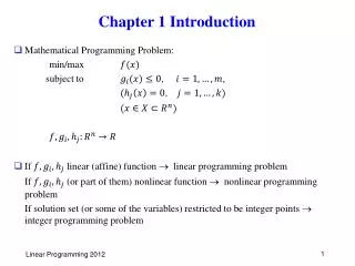
Chapter 1 Introduction. Mathematical Programming Problem: min/max subject to , , , If linear (affine) function linear programming problem If (or part of them) nonlinear function nonlinear programming problem

Mathematical Programming Problem: min/max subject to , , ,
E N D
Presentation Transcript
Chapter 1 Introduction • Mathematical Programming Problem: min/max subject to , , , • If linear (affine) function linear programming problem If (or part of them) nonlinear function nonlinear programming problem If solution set (or some of the variables) restricted to be integer points integer programming problem
Linear programming: problem of optimizing (maximize or minimize) a linear (objective) function subject to linear inequality (and equality) constraints. • General form: {max, min} subject to , (There may exist variables unrestricted in sign) • inner product of two column vectors : If , , then are said to be orthogonal. In 3-D, the angle between the two vectors is 90 degrees. ( vectors are column vectors unless specified otherwise)
Big difference from systems of linear equations is the existence of objective function and linear inequalities (instead of equalities) • Much deeper theoretical results and applicability than systems of linear equations. • : (decision) variables : right-hand-side { , , } : ith constraint { , } 0 : nonnegativity (nonpositivity) constraint : objective function • Other terminology: feasible solution, feasible set (region), free (unrestricted) variable, optimal (feasible) solution, optimal cost, unbounded
Important submatrix multiplications • Interpretation of constraints: see as submatrix multiplication. A: matrix , where is i-th unit vector denote constraints as { , , }
Any LP can be expressed as min max min () and take negative of the optimal cost nonnegativity (nonpositivity) are special cases of inequalities which will be handled separately in the algorithms. Feasible solution set of LP can always be expressed as (or ) (called polyhedron, a set which can be described as a solution set of finitely many linear inequalities) • We may sometimes use max , form (especially, when we study polyhedron)
Standard form problems • Standard form : min , , Two view points: • Find optimal weights (nonnegative) from possible nonnegative linear combinations of columns of A to obtain b vector • Find optimal solution that satisfies linear equations and nonnegativity • Reduction to standard form Free (unrestricted) variable , , (slack variable) , (surplus variable)
Any (practical) algorithm can solve the LP problem in equality form only (except nonnegativity) • Modified form of the simplex method can solve the problem with free variables directly (without using difference of two variables). It gives more sensible interpretation of the behavior of the algorithm.
1.2 Formulation examples • See other examples in the text. • Minimum cost network flow problem Directed network , ( ) arc capacity , unit flow cost : net supply at node i ( > 0: supply node, < 0: demand node), (We may assume = 0) Find minimum cost transportation plan that satisfies supply, demand at each node and arc capacities. minimize subject to i = 1, …, n (out flow - in flow = net flow at node i) (some people use, in flow – out flow = net flow) , ,
Choosing paths in a communication network ( (fractional) multicommodity flow problem) • Multicommodity flow problem: Several commodities share the network. For each commodity, it is min cost network flow problem. But the commodities must share the capacities of the arcs. Generalization of min cost network flow problem. Many applications in communication, distribution / transportation systems • Several commodities case • Actually one commodity. But there are multiple origin and destination pairs of nodes (telecom, logistics, ..). Each origin-destination pair represent a commodity. • Given telecommunication network (directed) with arc set A, arc capacity bits/sec, , unit flow cost /bit , , demand bits/sec for traffic from node k to node l. Data can be sent using more than one path. Find paths to direct demands with min cost.
Decision variables: : amount of data with origin k and destination l that traverses link Let = if if 0 otherwise • Formulation (flow based formulation) minimize subject to , (out flow - in flow = net flow at node i for commodity from node k to node l) (The sum of all commodities should not exceed the capacity of link (i, j) )
Alternative formulation (path based formulation) Let K: set of origin-destination pairs (commodities) : demand of commodity P(k): set of all possible paths for sending commodity kK P(k;e): set of paths in P(k) that traverses arc eA E(p): set of links contained in path p Decision variables: : fraction of commodity k sent on path p minimize subject to for all , for all for all , where • If , it is a single path routing problem (path selection problem, integer multicommodity flow problem).
path based formulation has smaller number of constraints, but enormous number of variables. can be solved easily by column generation technique (later). Integer version is more difficult to solve. • Extensions: Network design - also determine the number and type of facilities to be installed on the links (and/or nodes) together with routing of traffic. • Variations: Integer flow. Bifurcation of traffic may not be allowed. Determine capacities and routing considering rerouting of traffic in case of network failure, Robust network design (data uncertainty), ...
Pattern classification (Linear classifier) Given m objects with feature vector . Objects belong to one of two classes. We know the class to which each sample object belongs. We want to design a criterion to determine the class of a new object using the feature vector. Want to find a vector with such that, if , then , and if , then . (if it is possible)
Find a feasible solution that satisfies , , for all sample objects i Is this a linear programming problem? ( no objective function, strict inequality in constraints)
Is strict inequality allowed in LP? consider min x, x > 0 no minimum point. only infimum of objective value exists • If the system has a feasible solution , we can make the difference of the values in the right hand side and in the left hand side large by using solution for M > 0 and large. Hence there exists a solution that makes the difference at least 1 if the system has a solution. Remedy: Use , , • Important problem in data mining with applications in target marketing, bankruptcy prediction, medical diagnosis, process monitoring, …
Variations • What if there are many choices of hyperplanes? any reasonable criteria? • What if there is no hyperplane separating the two classes? • Do we have to use only one hyperplane? • Use of nonlinear function possible? How to solve them? • SVM (support vector machine), convex optimization • More than two classes?
1.3 Piecewise linear convex objective functions • Some problems involving nonlinear functions can be modeled as LP. • Def: Function is called a convex function if for all and all [0, 1] . ( the domain may be restricted) f called concave if is convex (picture: the line segment joining and in is not below the locus of )
Def:,1, 2 0, 1+ 2 = 1 Then 1x + 2y is said to be a convex combination of x, y. Generally, , where and is a convex combination of the points . • Def: A set is convex if for any , we have for any , . Picture: , , (line segment joining lies in ) x (1 = 1) y (1 = 0)
If we have , (without ), it is called an affine combination of x and y. Picture: , , (1 is arbitrary) (line passing through points )
relation between convex function and convex set • Def:. Define epigraph of as epi = . • Then previous definition of convex function is equivalent to epi being a convex set. When dealing with convex functions, we frequently consider epi to exploit the properties of convex sets. • Consider operations on functions that preserve convexity and operations on sets that preserve convexity.
Example: Consider , (maximum of affine functions, called a piecewise linear convex function.)
Thm: Let be convex functions. Then is also convex. pf) =
Min of piecewise linear convex functions Minimize Subject to Minimize Subject to ,
Q: What can we do about finding maximum of a piecewise linear convex function? maximum of a piecewise linear concave function (can be obtained as minimum of affine functions)? Minimum of a piecewise linear concave function?
Convex function has a nice property such that a local minimum point is a global minimum point. (when domain is or convex set) (HW later) Hence finding the minimum of a convex function defined over a convex set is usually easy. But finding the maximum of a convex function is difficult to solve. Basically, we need to examine all local maximum points. Similarly, finding the maximum of a concave function is easy, but finding the minimum of a concave function is difficult.
Suppose we have in constraints, where is a piecewise linear convex function , Q: What about constraints ? Can it be modeled as LP? • Def:, is a convex function, The set is called the level set of . • level set of a convex function is a convex set. (HW later) solution set of LP is convex (easy) non-convex solution set can’t be modeled as LP.
Problems involving absolute values • Minimize subject to (assume ) More direct formulations than piecewise linear convex function is possible. (1) Min subject to , , (2) Min subject to (want if , if and , i.e., at most one of is positive in an optimal solution. guarantees that.)
Data Fitting • Regression analysis using absolute value function Given m data points , . Want to find that predicts results given with function . Want that minimizes prediction error for all . minimize subject to , ,
Alternative criterion minimize minimize subject to , , Quadratic error function can't be modeled as LP, but need calculus method (closed form solution)
Special case of piecewise linear objective function : separable piecewise linear objective function. function , is called separable if Approximation of nonlinear function. slope: 0
Express variable in the constraints as , where ,,, In the objective function, use : min Since we solve min problem, it is guaranteed that we get in an optimal solution implies have values at their upper bounds.
1.4 Graphical representation and solution • Let . Geometric intuition for the solution sets of
Let be a (any) point satisfying . Then Hence , where is any solution to , or . Similarly, for , . 0
min s.t., ,
Representing complex solution set in 2-D ( variables, equations (coefficient vectors are linearly independent), nonnegativity, and ) • See text sec. 1.5, 1.6 for more backgrounds