Reinforcement Learning

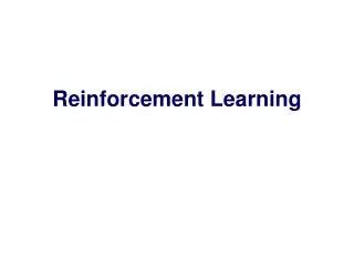
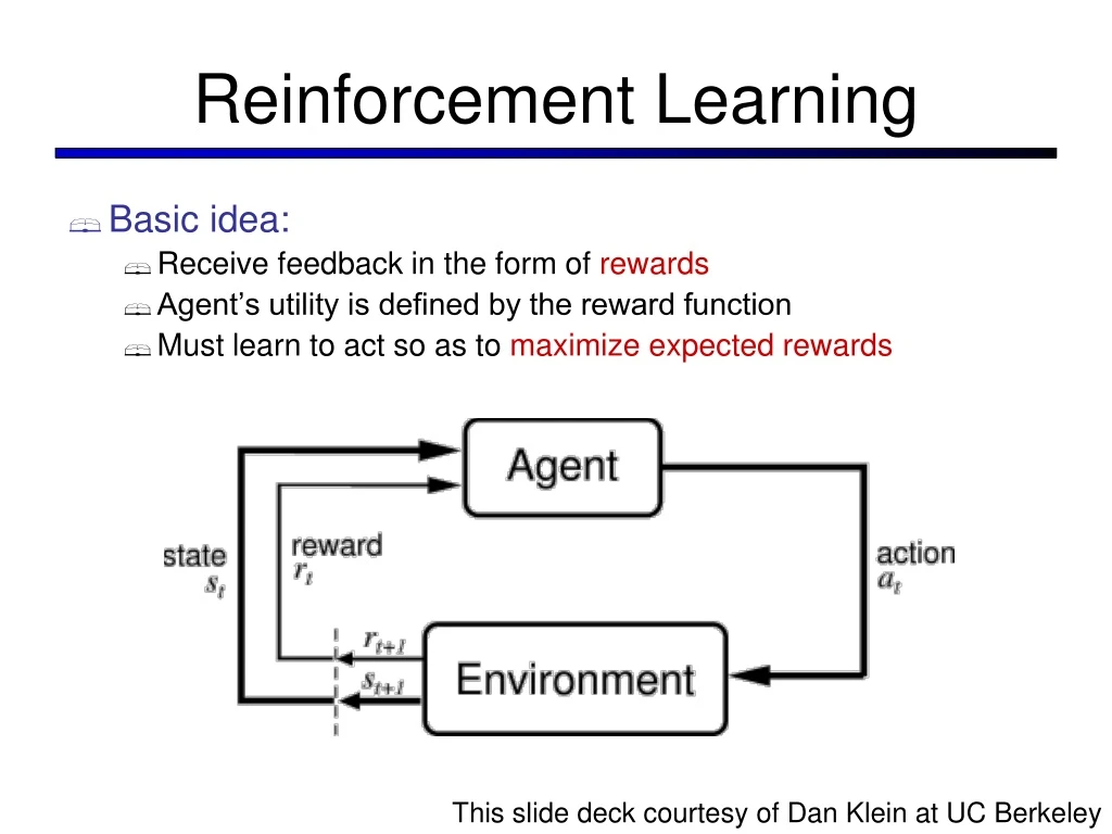
Reinforcement Learning • Basic idea: • Receive feedback in the form of rewards • Agent’s utility is defined by the reward function • Must learn to act so as to maximize expected rewards This slide deck courtesy of Dan Klein at UC Berkeley

s a s, a s,a,s’ s’ Recap: MDPs • Markov decision processes: • States S • Actions A • Transitions P(s’|s,a) (or T(s,a,s’)) • Rewards R(s,a,s’) (and discount ) • Start state s0 • Quantities: • Policy = map of states to actions • Episode = one run of an MDP • Utility = sum of discounted rewards • Values = expected future utility from a state • Q-Values = expected future utility from a q-state

Recap: Optimal Utilities • The utility of a state s: V*(s) = expected utility starting in s and acting optimally • The utility of a q-state (s,a): Q*(s,a) = expected utility starting in s, taking action a and thereafter acting optimally • The optimal policy: *(s) = optimal action from state s s is a state s a (s, a) is a q-state s, a (s,a,s’) is a transition s,a,s’ s’

s a s, a s,a,s’ s’ Recap: Bellman Equations • Definition of utility leads to a simple one-step lookahead relationship amongst optimal utility values: Total optimal rewards = maximize over choice of (first action plus optimal future) • Formally:

Practice: Computing Actions • Which action should we chose from state s: • Given optimal values V? • Given optimal q-values Q? • Lesson: actions are easier to select from Q’s!

Value Estimates • Calculate estimates Vk*(s) • Not the optimal value of s! • The optimal value considering only next k time steps (k rewards) • As k  , it approaches the optimal value • Almost solution: recursion (i.e. expectimax) • Correct solution: dynamic programming

Value Iteration • Idea: • Start with V0*(s) = 0, which we know is right (why?) • Given Vi*, calculate the values for all states for depth i+1: • Throw out old vector Vi* • Repeat until convergence • This is called a value update or Bellman update • Theorem: will converge to unique optimal values • Basic idea: approximations get refined towards optimal values • Policy may converge long before values do

Example: =0.9, living reward=0, noise=0.2 Example: Bellman Updates max happens for a=right, other actions not shown

Example: Value Iteration V2 V3 • Information propagates outward from terminal states and eventually all states have correct value estimates

0.705 Eventually: Correct Values V3 (when R=0, =0.9) V* (when R=-.04, =1) • This is the unique solution to the Bellman Equations 0.52 0.78 0.812 0.868 0.918 0.43 0.660 0.762 0.655 0.611 0.388

Utilities for a Fixed Policy • Another basic operation: compute the utility of a state s under a fixed (generally non-optimal) policy • Define the utility of a state s, under a fixed policy : V(s) = expected total discounted rewards (return) starting in s and following  • Recursive relation (one-step look-ahead / Bellman equation): s (s) s, (s) s, (s),s’ s’

Policy Evaluation • How do we calculate the V’s for a fixed policy? • Idea one: turn recursive equations into updates • Idea two: it’s just a linear system, solve with Matlab (or whatever)

Policy Iteration • Alternative approach: • Step 1: Policy evaluation: calculate utilities for some fixed policy (not optimal utilities!) until convergence • Step 2: Policy improvement: update policy using one-step look-ahead with resulting converged (but not optimal!) utilities as future values • Repeat steps until policy converges • This is policy iteration • It’s still optimal! • Can converge faster under some conditions

Policy Iteration • Policy evaluation: with fixed current policy , find values with simplified Bellman updates: • Iterate until values converge • Policy improvement: with fixed utilities, find the best action according to one-step look-ahead

Comparison • Both compute same thing (optimal values for all states) • In value iteration: • Every pass (or “backup”) updates both utilities (explicitly, based on current utilities) and policy (implicitly, based on current utilities) • Tracking the policy isn’t necessary; we take the max • In policy iteration: • Several passes to update utilities with fixed policy • After policy is evaluated, a new policy is chosen • Together, these are dynamic programming for MDPs

Asynchronous Value Iteration* • In value iteration, we update every state in each iteration • Actually, any sequences of Bellman updates will converge if every state is visited infinitely often • In fact, we can update the policy as seldom or often as we like, and we will still converge • Idea: Update states whose value we expect to change: If is large then update predecessors of s

Reinforcement Learning • Reinforcement learning: • Still have an MDP: • A set of states s  S • A set of actions (per state) A • A model T(s,a,s’) • A reward function R(s,a,s’) • Still looking for a policy (s) • New twist: don’t know T or R • I.e. don’t know which states are good or what the actions do • Must actually try actions and states out to learn

Example: Animal Learning • RL studied experimentally for more than 60 years in psychology • Rewards: food, pain, hunger, drugs, etc. • Mechanisms and sophistication debated • Example: foraging • Bees learn near-optimal foraging plan in field of artificial flowers with controlled nectar supplies • Bees have a direct neural connection from nectar intake measurement to motor planning area

Example: Backgammon • Reward only for win / loss in terminal states, zero otherwise • TD-Gammon learns a function approximation to V(s) using a neural network • Combined with depth 3 search, one of the top 3 players in the world • You could imagine training Pacman this way… • … but it’s tricky! (It’s also P3)

Passive Learning • Simplified task • You don’t know the transitions T(s,a,s’) • You don’t know the rewards R(s,a,s’) • You are given a policy (s) • Goal: learn the state values (and maybe the model) • I.e., policy evaluation • In this case: • Learner “along for the ride” • No choice about what actions to take • Just execute the policy and learn from experience • We’ll get to the active case soon • This is NOT offline planning!

Example: Direct Estimation y • Episodes: +100 (1,1) up -1 (1,2) up -1 (1,2) up -1 (1,3) right -1 (2,3) right -1 (3,3) right -1 (3,2) up -1 (3,3) right -1 (4,3) exit +100 (done) (1,1) up -1 (1,2) up -1 (1,3) right -1 (2,3) right -1 (3,3) right -1 (3,2) up -1 (4,2) exit -100 (done) -100 x  = 1, R = -1 V(2,3) ~ (96 + -103) / 2 = -3.5 V(3,3) ~ (99 + 97 + -102) / 3 = 31.3

Model-Based Learning • Idea: • Learn the model empirically through experience • Solve for values as if the learned model were correct • Simple empirical model learning • Count outcomes for each s,a • Normalize to give estimate of T(s,a,s’) • Discover R(s,a,s’) when we experience (s,a,s’) • Solving the MDP with the learned model • Iterative policy evaluation, for example s (s) s, (s) s, (s),s’ s’

Example: Model-Based Learning y • Episodes: +100 (1,1) up -1 (1,2) up -1 (1,2) up -1 (1,3) right -1 (2,3) right -1 (3,3) right -1 (3,2) up -1 (3,3) right -1 (4,3) exit +100 (done) (1,1) up -1 (1,2) up -1 (1,3) right -1 (2,3) right -1 (3,3) right -1 (3,2) up -1 (4,2) exit -100 (done) -100 x  = 1 T(<3,3>, right, <4,3>) = 1 / 3 T(<2,3>, right, <3,3>) = 2 / 2

Model-Free Learning • Want to compute an expectation weighted by P(x): • Model-based: estimate P(x) from samples, compute expectation • Model-free: estimate expectation directly from samples • Why does this work? Because samples appear with the right frequencies!

Sample-Based Policy Evaluation? • Who needs T and R? Approximate the expectation with samples (drawn from T!) s (s) s, (s),s’ s, (s) s’ s1’ s3’ s2’ Almost! But we only actually make progress when we move to i+1.

Temporal-Difference Learning • Big idea: learn from every experience! • Update V(s) each time we experience (s,a,s’,r) • Likely s’ will contribute updates more often • Temporal difference learning • Policy still fixed! • Move values toward value of whatever successor occurs: running average! s (s) s, (s) s’ Sample of V(s): Update to V(s): Same update:

Reinforcement Learning