Download
1 / 62
1.06k likes | 2.22k Views
Data Mining: Concepts and Techniques — Chapter 9 — Graph mining and Social Network Analysis. Li Xiong Slides credits: Jiawei Han and Micheline Kamber. Graph Mining and Social Network Analysis. Graph mining Frequent subgraph mining Social network analysis Social network

E N D
Data Mining: Concepts and Techniques— Chapter 9 —Graph mining and Social Network Analysis Li Xiong Slides credits: Jiawei Han and Micheline Kamber
Graph Mining and Social Network Analysis • Graph mining • Frequent subgraph mining • Social network analysis • Social network • Social network analysis at different levels • Link analysis Mining and Searching Graphs in Graph Databases
Graph Mining • Methods for Mining Frequent Subgraphs • Applications: • Graph Indexing • Similarity Search • Classification and Clustering • Summary Mining and Searching Graphs in Graph Databases
Why Graph Mining? • Graphs are ubiquitous • Chemical compounds (Cheminformatics) • Protein structures, biological pathways/networks (Bioinformactics) • Program control flow, traffic flow, and workflow analysis • XML databases, Web, and social network analysis • Graph is a general model • Trees, lattices, sequences, and items are degenerated graphs • Diversity of graphs • Directed vs. undirected, labeled vs. unlabeled (edges & vertices), weighted, with angles & geometry (topological vs. 2-D/3-D) • Complexity of algorithms: many problems are of high complexity Mining and Searching Graphs in Graph Databases
Graph, Graph, Everywhere from H. Jeong et al Nature 411, 41 (2001) Aspirin Yeast protein interaction network Co-author network Internet Mining and Searching Graphs in Graph Databases
Graph Pattern Mining • Frequent subgraph mining • Finding frequent subgraphs within a single graph • Finding frequent (sub)graphs in a set of graphs • support (occurrence frequency) no less than a minimum support threshold • Applications of graph pattern mining • Mining biochemical structures, program control flow analysis, XML structures or Web communities • Building blocks for graph classification, clustering, compression, comparison, and correlation analysis Mining and Searching Graphs in Graph Databases
Example: Frequent Subgraph Mining in Chemical Compounds GRAPH DATASET (A) (B) (C) FREQUENT PATTERNS (MIN SUPPORT IS 2) (1) (2) Mining and Searching Graphs in Graph Databases
Graph Mining Algorithms • Finding interesting and frequent substructures in a single graph • SUBDUE • Finding frequent patterns in a set of independent graphs • Apriori-based approach • Pattern-growth approach Mining and Searching Graphs in Graph Databases
SUBDUE (Holder et al. KDD’94) • Problem • Finding “interesting” and repetitive substructures (connected subgraphs) in data represented as a graph • Basic idea • Minimum description length (MDL) principle • Beam search algorithm • Start with best single vertices • Expand best substructures with a new edge • Substructures are evaluated based on their ability to compress input graphs Li Xiong
T1 C1 S1 S1 S1 S1 S1 Triangle T2 T3 T4 Square S2 S3 S4 Minimum Description Length (MDL) • Minimum description length (MDL) principle • A formalization of Occam’s Razor • Best hypothesis minimizes description length of the data (largest compression) • Graph substructure discovery based on MDL • Description length (DL): represent vertices and adjacency matrix • Graph compression: replace substructure instances with pointers • Find best substructure S in G that minimizes: DL(S) + DL(G|S) Input Database (G) Substructure (S1) Compressed Database (G|S1) C1 R1 R1 Holder et al.
Beam Search Algorithm • Beam search • An optimization of best-first search • Breadth-first search with a predetermined number of paths kept as candidates (beam width) • Subgraph discovery based on beam search • Start with best single vertices • Expand best substructures with a new edge • Substructures are evaluated based on their ability to compress input graphs (minimize description length) Li Xiong
triangle on circle square on on rectangle T1 on on on C1 S1 triangle triangle triangle on on on square T2 square square T3 T4 S2 S3 S4 Algorithm • Create substructure for each unique vertex label Input Database (G) (Graph form) Input Database (G) Substructures (S) triangle (4), square (4), circle (1), rectangle (1) R1 Holder et al.
triangle triangle on on circle square square on on rectangle on on on triangle triangle triangle rectangle on on on on circle square square square square triangle on on rectangle rectangle Algorithm (cont.) • Expand best substructures by an edge or edge + neighboring vertex Substructures (S)
Algorithm (cont.) • Keep best beam-width substructures on queue • Terminate when queue is empty or #discovered substructures >= limit • Compress graph with hierarchical description SRL Workshop
Frequent Subgraph Mining Approaches • Problem: finding frequent subgraphs in a set of graphs • Apriori-based approach • AGM: Inokuchi, et al. (PKDD’00) • FSG: Kuramochi and Karypis (ICDM’01) • PATH#: Vanetik and Gudes (ICDM’02, ICDM’04) • FFSM: Huan, et al. (ICDM’03) • Pattern growth approach • MoFa, Borgelt and Berthold (ICDM’02) • gSpan: Yan and Han (ICDM’02) • Gaston: Nijssen and Kok (KDD’04) • Close pattern mining • CLOSEGRAPH: Yan & Han (KDD’03) Mining and Searching Graphs in Graph Databases
Apriori-Based Approach • Level-wise algorithm: building candidate subgraphs from small frequent subgraphs Subgraphs with extra vertex, edge Frequent subgraphs G1 G G2 G’ … G’’ Gn JOIN
Apriori-Based Search • AGM (Apriori-based Graph Mining), Inokuchi, et al. PKDD’00 • generates new graphs with one more node • FSG (Frquent SubGraph mining), Kuramochi and Karypis, ICDM’01 • generates new graphs with one more edge b c a a a a a a a a Mining and Searching Graphs in Graph Databases
… … Pattern Growth Method (k+2)-edge (k+1)-edge G1 duplicate graph k-edge G2 G … Gn Mining and Searching Graphs in Graph Databases
GSPAN (Yan and Han ICDM’02) • Depth-based search and right-most extension Mining and Searching Graphs in Graph Databases
Graph Mining • Methods for Mining Frequent Subgraphs • Applications: • Classification and Clustering • Graph Indexing • Similarity Search Mining and Searching Graphs in Graph Databases
Using Graph Patterns • Similarity measures based on graph patterns • Feature-based similarity measure • Each graph is represented as a feature vector • Frequent subgraphs can be used as features • Vector distance • Structure-based similarity measure • Maximal common subgraph • Graph edit distance: insertion, deletion, and relabel • Frequent and discriminative subgraphs are high-quality indexing features Mining and Searching Graphs in Graph Databases
Social Network Analysis • Social network • Different levels of social network analysis • Common measures and methods for social network analysis • Link analysis Mining and Searching Graphs in Graph Databases
Social Network • Social network: a social structure consists of nodes and ties. • Nodes are the individual actors within the networks • May be different kinds • May have attributes, labels or classes • Ties are the relationships between the actors • May be different kinds • Links may have attributes, directed or undirected • Homogeneous networks • Single object type and single link type • Single model social networks (e.g., friends) • WWW: a collection of linked Web pages • Heterogeneous networks • Multiple object and link types • Medical network: patients, doctors, disease, contacts, treatments • Bibliographic network: publications, authors, venues Mining and Searching Graphs in Graph Databases
Small World Phenomenon • Number of degrees of separation in actual social networks? • Six-degree separation: everyone is an average of six "steps" away from each person on Earth. • Empirical studies • Michael Gurevich,1961. US population linked by 2 intermediaries • Duncan Watts, 2001. Email-delivery on the internet: average number of intermediaries is 6. • Leskovec and Horvitz, 2007. Instant messages: average path length is 6.6 September 19, 2014 24 Mining and Searching Graphs in Graph Databases
Six Degrees of Kevin Bacon Vertices: actors and actresses Edge between u and v if they appeared in a film together Kevin Bacon No. of movies : 46 No. of actors : 1811 Average separation: 2.79 876 Kevin Bacon 2.786981 46 1811 Is Kevin Bacon the most connected actor? NO! September 19, 2014 25 Data Mining: Concepts and Techniques
Bacon-map #876 Kevin Bacon #1 Rod Steiger Donald Pleasence #2 September 19, 2014 #3 Martin Sheen 26 Data Mining: Concepts and Techniques
Social Network Analysis • Actor level: centrality, prestige, and roles such as isolates, liaisons, bridges, etc. • Dyadic level: distance and reachability, structural and other notions of equivalence, and tendencies toward reciprocity. • Triadic level: balance and transitivity • Subset level: cliques, cohesive subgroups, components • Network level: connectedness, diameter, centralization, density, prestige, etc. Social network analysis: methods and applications
Measures in Social Network Analysis – Actor level • Non-directional graphs • Degree Centrality • The number of direct connections a node has • 'connector' or 'hub' in this network • Betweenness Centrality • Degree an individual lies between other individuals in the network • an intermediary; liaison; bridge • Closeness Centrality • The degree an individual is near all other individuals in a network (directly or indirectly) • Eigenvector centrality • A measure of relative importance of a node • Based on the principle that connections to nodes having a high score contribute more to the current node • Directional graphs • Prestige: measure the degree of incoming ties Mining and Searching Graphs in Graph Databases
Actor Centrality Example OrgNet.com
Measures in Social Network Analysis – Dyadic, Triadic and Subset Level • Path Length • The distances between pairs of nodes in the network. • Structural equivalence • Extent to which actors have a common set of linkages to other actors in the system. • Clustering coefficient • A measure of the likelihood that two associates of a node are associates themselves • Cliquishness of u’s neighborhood • Cohesion • The degree to which actors are connected directly to each other by cohesive bonds • Cliques Mining and Searching Graphs in Graph Databases
Measures in Social Network Analysis – Network Level • Network Centralization • The difference between number of links for each node • Centralized vs. decentralized networks • Network density • Proportion of ties in a network relative to the total number possible • Sparse vs. dense networks • Average Path Length • Average of distances between all pairs of nodes • Reach • The degree any member of a network can reach other members of the network. • Structural cohesion • The minimum number of members who, if removed from a group, would disconnect the group. Mining and Searching Graphs in Graph Databases
Another Taxonomy of Link Mining Tasks • Object-Related Tasks • Link-based object ranking • Link-based object classification • Object clustering (group detection) • Object identification (entity resolution) • Link-Related Tasks • Link prediction • Graph-Related Tasks • Subgraph discovery • Graph classification • Generative model for graphs Data Mining: Concepts and Techniques
Social Network Applications • Link-based object ranking for WWW (actor-level analysis) • PageRank • HITS • Influence and diffusion Mining and Searching Graphs in Graph Databases
Link-Based Object Ranking (LBR) • Exploit the link structure of a graph to order or prioritize the set of objects within the graph • Focused on graphs with single object type and single link type • Focus of link analysis community • Algorithms • PageRank • HITS Data Mining: Concepts and Techniques
PageRank: Ranking web pages (Brin & Page’98) • Intuition • Web pages are not equally “important” • www.joe-schmoe.com v www.stanford.edu • Links as citations: a page cited often is more important • www.stanford.edu has 23,400 inlinks • www.joe-schmoe.com has 1 inlink • Are all links equal? • Recursive model: being cited by a highly cited paper counts a lot… • Eigenvector prestige measure
Yahoo Amazon M’soft Simple Recursive Flow Model • Each link’s vote is proportional to the importance of its source page • If page P with importance x has n outlinks, each link gets x/n votes • Page P’s own importance is the sum of the votes on its inlinks y/2 y y = y /2 + a /2 a = y /2 + m m = a /2 a/2 y/2 m • Solving the equation with constraint: y+a+m = 1 • y = 2/5, a = 2/5, m = 1/5 a/2 m a
j i = M r Matrix formulation • Web link matrix M: one row and one column per web page • Suppose page j has n outlinks, if j ! i, then Mij=1/n, else Mij=0 • M is a columnstochastic matrix - Columns sum to 1 • Rank vector r: one entry per web page • ri is the importance score of page i • |r| = 1 • Flow equation: r = Mr • Rank vector is an eigenvector of the web matrix i j r
Yahoo r = Mr Amazon M’soft y 1/2 1/2 0 y a = 1/2 0 1 a m 0 1/2 0 m Matrix formulation Example y a m y 1/2 1/2 0 a 1/2 0 1 m 0 1/2 0 y = y /2 + a /2 a = y /2 + m m = a /2
Power Iteration method • Simple iterative scheme (aka relaxation) • Suppose there are N web pages • Initialize: r0 = [1/N,….,1/N]T • Iterate: rk+1 = Mrk • Stop when |rk+1 - rk|1 < • |x|1 = 1≤i≤N|xi| is the L1 norm • Can use any other vector norm e.g., Euclidean
Yahoo Amazon M’soft Power Iteration Example y a m y 1/2 1/2 0 a 1/2 0 1 m 0 1/2 0 y a = m 1/3 1/3 1/3 1/3 1/2 1/6 5/12 1/3 1/4 3/8 11/24 1/6 2/5 2/5 1/5 . . .
Random Walk Interpretation • Imagine a random web surfer • At any time t, surfer is on some page P • At time t+1, the surfer follows an outlink from P uniformly at random • Ends up on some page Q linked from P • Process repeats indefinitely • p(t) is the probability distribution whose ith component is the probability that the surfer is at page i at time t
The stationary distribution • Where is the surfer at time t+1? • p(t+1) = Mp(t) • Suppose the random walk reaches a state such that p(t+1) = Mp(t) = p(t) • Then p(t) is a stationary distribution for the random walk • Our rank vector r satisfies r = Mr
Existence and Uniqueness of the Solution • Theory of random walks (aka Markov processes): For graphs that satisfy certain conditions, the stationary distribution is unique and eventually will be reached no matter what the initial probability distribution at time t = 0. Mining and Searching Graphs in Graph Databases
Spider traps • A group of pages is a spider trap if there are no links from within the group to outside the group • Spider traps violate the conditions needed for the random walk theorem Yahoo y a m y 1/2 1/2 0 a 1/2 0 0 m 0 1/2 1 Amazon M’soft y a = m 1 1 1 1 1/2 3/2 3/4 1/2 7/4 5/8 3/8 2 0 0 3 . . .
Random teleports • At each time step, the random surfer has two options: • With probability , follow a link at random • With probability 1-, jump to some page uniformly at random • Common values for are in the range 0.8 to 0.9 • Surfer will teleport out of spider trap within a few time steps
Random teleports Example ( = 0.8) 1/2 1/2 0 1/2 0 0 0 1/2 1 1/3 1/3 1/3 1/3 1/3 1/3 1/3 1/3 1/3 + 0.2 Yahoo 0.8 y 7/15 7/15 1/15 a 7/15 1/15 1/15 m 1/15 7/15 13/15 Amazon M’soft y a = m 1 1 1 1.00 0.60 1.40 0.84 0.60 1.56 0.776 0.536 1.688 7/11 5/11 21/11 . . .
Matrix formulation • Matrix vector A • Aij = Mij + (1-)/N • Mij = 1/|O(j)| when j!i and Mij = 0 otherwise • Verify that A is a stochastic matrix • The page rank vectorr is the principal eigenvector of this matrix • satisfying r = Ar • Equivalently, r is the stationary distribution of the random walk with teleports
HITS: Capturing Authorities & Hubs (Kleinberg’98) • Intuitions • Pages that are widely cited are good authorities • Pages that cite many other pages are good hubs • HITS (Hypertext-Induced Topic Selection) • Authorities are pages containing useful information and linked by Hubs • course home pages • home pages of auto manufacturers • Hubs are pages that link to Authorities • course bulletin • list of US auto manufacturers • Iterative reinforcement … Hubs Authorities Data Mining: Concepts and Techniques
Matrix Formulation • Transition (adjacency) matrix A • A[i, j] = 1 if page i links to page j, 0 if not • The hub score vector h: score is proportional to the sum of the authority scores of the pages it links to • h = λAa • Constant λ is a scale factor • The authority score vector a: score is proportional to the sum of the hub scores of the pages it is linked from • a = μAT h • Constant μ is scale factor Hubs Authorities
Transition Matrix Example y a m Yahoo y 1 1 1 a 1 0 1 m 0 1 0 A = Amazon M’soft