Download
1 / 80
840 likes | 1.1k Views
Structural Variation in the Human Genome Michael Snyder March 2, 2010. Single nucleotide polymorphisms (SNPs). GATTTAGATC G CGATAGAG GATTTAGATC T CGATAGAG. Genetic Variation Among People. 0.1% difference among people. Mapping Structural Variation in Humans. >1 kb segments.

E N D
Structural Variation in the Human GenomeMichael SnyderMarch 2, 2010
Single nucleotide polymorphisms (SNPs) GATTTAGATCGCGATAGAG GATTTAGATCTCGATAGAG Genetic Variation Among People 0.1% difference among people
Mapping Structural Variation in Humans >1 kb segments • Thought to be Common • 12% of the genome • (Redon et al. 2006) • Likely involved in phenotype • variation and disease • Until recently most methods for • detection were low resolution (>50 kb) CNVs
Why Study Structural Variation? Common in “normal” human genomes--major cause of phenotypic variation Common in certain diseases, particularly cancer Now showing up in rare disease; autism, schizophrenia
Why Not Studied More? Often involves repeated regions Rearrangements are complex Can involve highly repetitive elements
Genome Tiling Arrays 800 bp 25-36mer
High-Resolution CGH with Oligonucleotide Tiling Microarrays HR-CGH Maskless Array Synthesis 385,000 oligomers/chip Isothermal oligomers, 45-85 bp Tiling at ~1/100bp non-repetitive genomic sequence Detects CNVs at <1 kb resolution Urban et al., 2006 With R. Selzer and R. Green
Patient 98-135 Patient 99-199 Patient 97-237 LCR A B C D High Resolution Comparative Genomic Hybridization Chromosome 22 Chromosome 22 Nimblegen/MAS Technology Isothermal Arrays Covering Chromosome 22 Mapped Copy Number Variation In VCFS Patients Resolution ~50-200 bp Urban et al. (2006) PNAS
Mapping Breakpoints of Partial Trisomies of Chromosome 21 verified verified With Korenberg Lab, UCLA
Copy Number Variations in the Human Genome Signal Person 1 Signal Person 2 Chromosome Position Extra DNA Missing DNA
800 bp PCR Products Oligonucleotide Array 36mer Genome Tiling Arrays Massively Parallel Sequencing AGTTCACCTAAGA… CTTGAATGCCGAT… GTCATTCCGCAAT…
High Throughput DNA Sequencing based Methods to detect CNVs/SVs 1. Paired ends Deletion Reference Mapping Genome Reference Sequenced paired-ends 3. Split read 2. Read depth Deletion Deletion Reference Reference Genome Genome Read Reads Mapping Mapping Read count Reference Zero level
High Resolution-Paired-End Mapping (HR-PEM) Bio Bio Bio Bio • Shear to 3 kb • Adaptor ligation • Circularize Bio Bio Genomic DNA Fragments Random Cleavage 200-300bp 454 Sequencing (250bp reads, 400K reads/run) Map paired ends to reference genome Korbel et al., 2007 Science
Summary of PEM Results *at this resolution
~1000 SVs >2.5kb per Person * VCFS *
Cumulative sequence coverage in Mb (NA18505, shown as function of SV-size) Size distribution of Structural Variants 10kb [Compare with overall 11M refSNP entries] [Arrow indicates lower size cutoff for deletions]
Cumulative sequence coverage in Mb (NA18505, shown as function of SV-size) 10kb Size distribution of Structural Variants 10kb [Compare with overall 11M refSNP entries] [Arrow indicates lower size cutoff for deletions]
? + + + Genome Sequencer FLX High Throughput Sequencing of Breakpoints Cut Gel Bands and Pool PCR SVs Shotgun-sequence PCR Mixture Using 454 Assemble contigs and determine breakpoints >200 SVs Sequenced Across Breakpoints
Analysis of Breakpoints Homologous Recombination 14% Nonhomologous Recombination 56% Retrotransposons 30%
Non-allelic homologous recombination (NAHR; breakpoints in OR51A2 and OR51A4) 17% of SVs Affect Genes Olfactory Receptor Gene Fusion
Heterogeneity in Olfactory Receptor Genes (Examined 851 OR Loci) CNVs affect: 93 Genes 151 genes
Paired-end • Variations of the method are available for many platforms: Roche, Illumina, LifeTechnologies • Long reads are preferable for optimal detection • Can get different sizes - Roche 20 kb, 8kb, 3 kb - Ilumina, SOLiD 1.5 kb
Paired-end: Advantages/Disadvantages Can detect highly repetitive CNVs (LINE, SINE, etc.) Detect inversions as well as insertions and deletions Defines location of CNV Relies on confident independent mapping of each end, problems in regions flanked by repeats Small span between ends limits resolution of complex regions Large span between ends limits resolution of break points
High Throughput DNA Sequencing based Methods to detect CNVs/SVs 1. Paired ends Deletion Reference Mapping Genome Reference Sequenced paired-ends 3. Split read 2. Read depth Deletion Deletion Reference Reference Genome Genome Read Reads Mapping Mapping Read count Reference Zero level
Sequence Read Depth Analysis Individual sequence Reads Mapping Reference genome Counting mapped reads Read depth signal Zero level 28
Novel method, CNVnator,mean-shift approach Alexej Abyzov For each bin attraction (mean-shift) vector points in the direction of bins with most similar RD signal No prior assumptions about number, sizes, haplotype, frequency and density of CNV regions Achieves discontinuity-preserving smoothing Derived from image-processing applications
CNVnator on RD data NA12878, Solexa 36 bp paired reads, ~28x coverage
RD vs paired-end Read Depth Paired-end Difficulty in finding highly repetitive CNVs (LINE, SINE, etc.) Uncertain in CNV location Uses mutual information of both ends, better mapping and ascertainment in homologous region Ascertains complex regions Can find large insertions Can be used with paired-end, single-end and mixed data Can detect highly repetitive CNVs (LINE, SINE, etc.) Defines precise location of CNV Relies on confident independent mapping of each end, problems in regions flanked by repeats Small span between ends limits resolution of complex regions Large span between ends limits resolution of break points
RD vs read pair (example) Not found by short read pair analysis due to not confident read mapping Caucasian trio daughter
High Throughput DNA Sequencing based Methods to detect CNVs/SVs 1. Paired ends Deletion Reference Mapping Genome Reference Sequenced paired-ends 3. Split read 2. Read depth Deletion Deletion Reference Reference Genome Genome Read Reads Mapping Mapping Read count Reference Zero level
Split-read Analysis Deletion Event Reference Deletion Read Insertion Event Breakpoint Reference Read Insertion
Methods toFind SVs 1. Paired ends Deletion Reference Mapping Genome Reference Sequenced paired-ends 2. Split read 3. Read depth (or aCGH) Deletion Deletion Reference Reference Genome Genome Read Reads Mapping Mapping Read count Reference Zero level 4. Local Reassembly [Snyder et al. Genes & Dev. ('10), in press]
Simple Local Assembly: iterative contig extension -- a mostly greedy approach Du et al. (2009), PLoS Comp Biol.
BreakSeq enables detecting SVs in Next-Gen Sequencing data based on breakpoint junctions Detection of insertions Detection of deletions Leveraging read data to identify previously known SVs (“Break-Seq”) Map reads onto Library of SV breakpoint junctions [Lam et al. Nat. Biotech. ('10)]
Applying BreakSeq to short-read based personal genomes *According to the operational definition we used in our analysis (>1kb events) less than 5 SVs were previously reported in these genomes … [Lam et al. Nat. Biotech. ('10)]
Conclusions • SVs are abundant in the human genome • Different methods are used to detect them: Read pairs, Read Depth, Split reads, New assembly • Many SV breakpoints are being sequenced; nonhomologous end joining is common. The breakppoint library can be used to identify SVs.
Acknowledgments • Jan Korbel • Alexej Abyzov • Alex Urban • Zhengdong Zhang • Hugo Lam • Mark Gerstein 454 for Paired End Tim Harkins, Michael Egholm
2nd-Gen Sequencing based Methods to detect CNVs/SVs 1. Paired ends Deletion Reference Mapping Genome Reference Sequenced paired-ends 2. Split read 3. Read depth Deletion Deletion Reference Reference Genome Genome Read Reads Mapping Mapping Read count Reference Zero level
SV-CapSeq v1.0 results for deletions Combining 3 captures/elutions (1 per member of CEU trio) and 1+(2x0.5) 454 Titanium runs *For 2x allelic coverage and breakpoints at least 20 bp away from read ends
SV Junction and Identification [Lam et al. Nat. Biotech. ('10)]
Contents of the SV-CapSeq array v1.0 2.1 million oligomers tiling the target regions of the genome: 1839 deletion CNVs from (mostly) short read Solexa data (1000 Genome Project) From long read 454 paired-end data: 575 deletion CNVs 296 insertions CNVs 191 inversions SVs (plus Split-Read indel predictions, Zhengdong Zhang)
12,995,076 12,988,627 Array capture RD signal 12,988,735 12,996,115 PCR primers 12,988,825 12,994,750 Multi-method prediction Sequence Read Depth Read depth analysis Chromosome 7, Mbp ~6500 bp deletion CNV