Introduction to Algorithms Shortest Paths
Introduction to Algorithms Shortest Paths. CSE 680 Prof. Roger Crawfis. Shortest Path. Given a weighted directed graph, one common problem is finding the shortest path between two given vertices

Introduction to Algorithms Shortest Paths
E N D
Presentation Transcript
Introduction to AlgorithmsShortest Paths CSE 680 Prof. Roger Crawfis
Shortest Path • Given a weighted directed graph, one common problem is finding the shortest path between two given vertices • Recall that in a weighted graph, the length of a path is the sum of the weights of each of the edges in that path
Applications • One application is circuit design: the time it takes for a change in input to affect an output depends on the shortest path http://www.hp.com/
Shortest Path • Given the graph below, suppose we wish to find the shortest path from vertex 1 to vertex 13
Shortest Path • After some consideration, we may determine that the shortest path is as follows, with length 14 • Other paths exists, but they are longer
Negative Cycles • Clearly, if we have negative vertices, it may be possible to end up in a cycle whereby each pass through the cycle decreases the total length • Thus, a shortest length would be undefined for such a graph • Consider the shortest pathfrom vertex 1 to 4... • We will only consider non-negative weights.
2 23 3 9 s 18 14 6 2 6 4 19 30 11 5 15 5 6 16 20 t 7 44 Shortest Path Example • Given: • Weighted Directed graph G = (V, E). • Source s, destination t. • Find shortest directed path from s to t. Cost of path s-2-3-5-t = 9 + 23 + 2 + 16 = 48.
2 23 3 9 s 18 14 6 2 6 4 19 30 11 5 15 5 6 16 20 t 7 44 Discussion Items • How many possible paths are there from s to t? • Can we safely ignore cycles? If so, how? • Any suggestions on how to reduce the set of possibilities? • Can we determine a lower bound on the complexity like we did for comparison sorting?
Key Observation • A key observation is that if the shortest path contains the node v, then: • It will only contain v once, as any cycles will only add to the length. • The path from s to v must be the shortest path to v from s. • The path from v to t must be the shortest path to t from v. • Thus, if we can determine the shortest path to all other vertices that are incident to the target vertex we can easily compute the shortest path. • Implies a set of sub-problems on the graph with the target vertex removed.
Dijkstra’s Algorithm • Works when all of the weights are positive. • Provides the shortest paths from a source to all other vertices in the graph. • Can be terminated early once the shortest path to t is found if desired.
Shortest Path • Consider the following graph with positive weights and cycles.
Dijkstra’s Algorithm • A first attempt at solving this problem might require an array of Boolean values, all initially false, that indicate whether we have found a path from the source.
Dijkstra’s Algorithm • Graphically, we will denote this with check boxes next to each of the vertices (initially unchecked)
Dijkstra’s Algorithm • We will work bottom up. • Note that if the starting vertex has any adjacent edges, then there will be one vertex that is the shortest distance from the starting vertex. This is the shortest reachable vertex of the graph. • We will then try to extend any existing paths to new vertices. • Initially, we will start with the path of length 0 • this is the trivial path from vertex 1 to itself
Dijkstra’s Algorithm • If we now extend this path, we should consider the paths • (1, 2) length 4 • (1, 4) length 1 • (1, 5) length 8 The shortest path so far is (1, 4) which is of length 1.
Dijkstra’s Algorithm • Thus, if we now examine vertex 4, we may deduce that there exist the following paths: • (1, 4, 5) length 12 • (1, 4, 7) length 10 • (1, 4, 8) length 9
Dijkstra’s Algorithm • We need to remember that the length of that path from node 1 to node 4 is 1 • Thus, we need to store the length of a path that goes through node 4: • 5 of length 12 • 7 of length 10 • 8 of length 9
Dijkstra’s Algorithm • We have already discovered that there is a path of length 8 to vertex 5 with the path (1, 5). • Thus, we can safely ignore this longer path.
Dijkstra’s Algorithm • We now know that: • There exist paths from vertex 1 to vertices {2,4,5,7,8}. • We know that the shortest path from vertex 1 to vertex 4 is of length 1. • We know that the shortest path to the other vertices {2,5,7,8} is at most the length listed in the table to the right.
Dijkstra’s Algorithm • There cannot exist a shorter path to either of the vertices 1 or 4, since the distances can only increase at each iteration. • We consider these vertices to be visited If you only knew this information and nothing else about the graph, what is the possible lengths from vertex 1 to vertex 2? What about to vertex 7?
Relaxation • Maintaining this shortest discovered distance d[v] is called relaxation: Relax(u,v,w) { if (d[v] > d[u]+w) then d[v]=d[u]+w; } 2 2 9 6 5 5 v Relax v u Relax u 2 2 7 6 5 5
Dijkstra’s Algorithm • In Dijkstra’s algorithm, we always take the next unvisited vertex which has the current shortest path from the starting vertex in the table. • This is vertex 2
Dijkstra’s Algorithm • We can try to update the shortest paths to vertices 3 and 6 (both of length 5) however: • there already exists a path of length 8 < 10 to vertex 5 (10 = 4 + 6) • we already know the shortest path to 4 is 1
Dijkstra’s Algorithm • To keep track of those vertices to which no path has reached, we can assign those vertices an initial distance of either • infinity (∞ ), • a number larger than any possible path, or • a negative number • For demonstration purposes, we will use ∞
Dijkstra’s Algorithm • As well as finding the length of the shortest path, we’d like to find the corresponding shortest path • Each time we update the shortest distance to a particular vertex, we will keep track of the predecessor used to reach this vertex on the shortest path.
Dijkstra’s Algorithm • We will store a table of pointers, each initially 0 • This table will be updated eachtime a distance is updated
Dijkstra’s Algorithm • Graphically, we will display the reference to the preceding vertex by a red arrow • if the distance to a vertex is ∞, there will be no preceding vertex • otherwise, there will be exactly one preceding vertex
Dijkstra’s Algorithm • Thus, for our initialization: • we set the current distance to the initial vertex as 0 • for all other vertices, we set the current distance to ∞ • all vertices are initially marked as unvisited • set the previous pointer for all vertices to null
Dijkstra’s Algorithm • Thus, we iterate: • find an unvisited vertex which has the shortest distance to it • mark it as visited • for each unvisited vertex which is adjacent to the current vertex: • add the distance to the current vertex to the weight of the connecting edge • if this is less than the current distance to that vertex, update the distance and set the parent vertex of the adjacent vertex to be the current vertex
Dijkstra’s Algorithm • Halting condition: • we successfully halt when the vertex we are visiting is the target vertex • if at some point, all remaining unvisited vertices have distance ∞, then no path from the starting vertex to the end vertex exits • Note: We do not halt just because we have updated the distance to the end vertex, we have to visit the target vertex.
Example • Consider the graph: • the distances are appropriately initialized • all vertices are marked as being unvisited
Example • Visit vertex 1 and update its neighbours, marking it as visited • the shortest paths to 2, 4, and 5 are updated
Example • The next vertex we visit is vertex 4 • vertex 5 1 + 11 ≥ 8 don’t update • vertex 7 1 + 9 < ∞ update • vertex 8 1 + 8 < ∞ update
Example • Next, visit vertex 2 • vertex 3 4 + 1 < ∞ update • vertex 4 already visited • vertex 5 4 + 6 ≥ 8 don’t update • vertex 6 4 + 1 < ∞ update
Example • Next, we have a choice of either 3 or 6 • We will choose to visit 3 • vertex 5 5 + 2 < 8 update • vertex 6 5 + 5 ≥ 5 don’t update
Example • We then visit 6 • vertex 8 5 + 7 ≥ 9 don’t update • vertex 9 5 + 8 < ∞ update
Example • Next, we finally visit vertex 5: • vertices 4 and 6 have already been visited • vertex 7 7 + 1 < 10 update • vertex 8 7 + 1 < 9 update • vertex 9 7 + 8 ≥ 13 don’t update
Example • Given a choice between vertices 7 and 8, we choose vertex 7 • vertices 5 has already been visited • vertex 8 8 + 2 ≥ 8 don’t update
Example • Next, we visit vertex 8: • vertex 9 8 + 3 < 13 update
Example • Finally, we visit the end vertex • Therefore, the shortest path from 1 to 9 has length 11
Example • We can find the shortest path by working back from the final vertex: • 9, 8, 5, 3, 2, 1 • Thus, the shortest path is (1, 2, 3, 5, 8, 9)
Example • In the example, we visited all vertices in the graph before we finished • This is not always the case, consider the next example
Example • Find the shortest path from 1 to 4: • the shortest path is found after only three vertices are visited • we terminated the algorithm as soon as we reached vertex 4 • we only have useful information about 1, 3, 4 • we don’t have the shortest path to vertex 2
Dijkstra’s algorithm • d[s] 0 • for each vÎV – {s} • dod[v] ¥ • S • Q V ⊳Q is a priority queue maintainingV – S • whileQ ¹ • dou EXTRACT-MIN(Q) • S SÈ {u} • for each vÎAdj[u] • doif d[v] > d[u] + w(u, v) • then d[v] d[u] + w(u, v) • p[v] u
Dijkstra’s algorithm • d[s] 0 • for each vÎV – {s} • dod[v] ¥ • S • Q V ⊳Q is a priority queue maintainingV – S • whileQ ¹ • dou EXTRACT-MIN(Q) • S SÈ {u} • for each vÎAdj[u] • doif d[v] > d[u] + w(u, v) • then d[v] d[u] + w(u, v) • p[v] u relaxation step Implicit DECREASE-KEY
Example of Dijkstra’s algorithm 2 Graph with nonnegative edge weights: B D 10 8 A 1 4 7 9 3 C E 2
Example of Dijkstra’s algorithm ¥ ¥ Initialize: 2 B D 10 8 A 0 1 4 7 9 3 C E Q: A B C D E 2 ¥ ¥ ¥ ¥ 0 ¥ ¥ S: {}
Example of Dijkstra’s algorithm ¥ ¥ “A”EXTRACT-MIN(Q): 2 B D 10 8 A 0 1 4 7 9 3 C E Q: A B C D E 2 ¥ ¥ ¥ ¥ 0 ¥ ¥ S: { A }
Example of Dijkstra’s algorithm ¥ 10 Relax all edges leaving A: 2 B D 10 8 A 0 1 4 7 9 3 C E Q: A B C D E 2 ¥ ¥ ¥ ¥ 0 ¥ 3 3 ¥ ¥ 10 S: { A }
Example of Dijkstra’s algorithm ¥ 10 “C”EXTRACT-MIN(Q): 2 B D 10 8 A 0 1 4 7 9 3 C E Q: A B C D E 2 ¥ ¥ ¥ ¥ 0 ¥ 3 3 ¥ ¥ 10 S: { A, C }