Classification Techniques for Microarray Data
This lecture focuses on the classification problem in microarray data, exploring key concepts, algorithms, and evaluation methods. We will examine learning sets related to prognosis in cancer, using examples like the gene expression profiling of breast cancer by L. van’t Veer et al. and the molecular classification of cancer by Golub et al. Additionally, we will cover support vector machines (SVMs) and k-nearest neighbors (KNN), their methodologies, advantages, and challenges. Join us to delve into state-of-the-art techniques for bioinformatics classification tasks.

Classification Techniques for Microarray Data
E N D
Presentation Transcript
CSCE555 Bioinformatics • Lecture 15 classification for microarray data Meeting: MW 4:00PM-5:15PM SWGN2A21 Instructor: Dr. Jianjun HuCourse page: http://www.scigen.org/csce555 University of South Carolina Department of Computer Science and Engineering 2008 www.cse.sc.edu.
Outline • Classification problem in microarray data • Classification concepts and algorithms • Evaluation of classification algorithms • Summary
Learning set Bad prognosis recurrence < 5yrs Good Prognosis recurrence > 5yrs ? Good Prognosis Matesis > 5 Predefine classes Clinical outcome Objects Array Feature vectors Gene expression new array Reference L van’t Veer et al (2002) Gene expression profiling predicts clinical outcome of breast cancer. Nature, Jan. . Classification rule
Learning set Predefine classes Tumor type B-ALL T-ALL AML T-ALL ? Objects Array Feature vectors Gene expression new array Reference Golub et al (1999) Molecular classification of cancer: class discovery and class prediction by gene expression monitoring. Science 286(5439): 531-537. Classification Rule
Classification/Discrimination Y Normal Normal Normal Cancer Cancer unknown =Y_new • Each object (e.g. arrays or columns)associated with a class label (or response) Y {1, 2, …, K} and a feature vector (vector of predictor variables) of G measurements: X = (X1, …, XG) • Aim: predict Y_new from X_new. sample1 sample2 sample3 sample4 sample5 … New sample 1 0.46 0.30 0.80 1.51 0.90 ... 0.34 2 -0.10 0.49 0.24 0.06 0.46 ... 0.43 3 0.15 0.74 0.04 0.10 0.20 ... -0.23 4 -0.45 -1.03 -0.79 -0.56 -0.32 ... -0.91 5 -0.06 1.06 1.35 1.09 -1.09 ... 1.23 X X_new
Basic principles of discrimination • Each object associated with a class label (or response) Y {1, 2, …, K} and a feature vector (vector of predictor variables) of G measurements: X = (X1, …, XG) • Aim:predict Y from X. Predefined Class {1,2,…K} K 1 2 Objects Y = Class Label = 2 X = Feature vector {colour, shape} Classification rule ? X = {red, square} Y = ?
KNN: Nearest neighbor classifier • Based on a measure of distance between observations (e.g. Euclidean distance or one minus correlation). • k-nearest neighbor rule (Fix and Hodges (1951)) classifies an observation X as follows: • find thek observations in the learning set closestto X • predict the class of X by majority vote, i.e., choose the class that is most common among those k observations. • The number of neighbors kcan be chosen by cross-validation(more on this later).
3-Nearest Neighbors query point qf 3 nearest neighbors 2x,1o
SVM: Support Vector Machines • SVMs are currently among the best performers for a number of classification tasks ranging from text to genomic data. • In order to discriminate between two classes, given a training dataset • Map the data to a higher dimension space (feature space) • Separate the two classes using an optimal linear separator
Key Ideas of SVM: Margins of Linear Separators Maximum margin linear classifier
ρ Optimal hyperplane Support vectors uniquely characterize optimal hyper-plane margin Optimal hyper-plane Support vector
Finding the Support Vectors Lagrangian multiplier method for constrained opt Inner product of vectors
Key Ideas of SVM: Feature Space Mapping • Map the original data to some higher-dimensional feature space where the training set is linearly separable: Φ: x→φ(x) (x1,x2) (x1,x2, x1^2, x2^2, x1*x2, …)
The “Kernel Trick” • The linear classifier relies on inner product between vectors K(xi,xj)=xiTxj • If every datapoint is mapped into high-dimensional space via some transformation Φ: x→φ(x), the inner product becomes: K(xi,xj)= φ(xi)Tφ(xj) • A kernel function is some function that corresponds to an inner product in some expanded feature space. • Example: 2-dimensional vectors x=[x1 x2]; let K(xi,xj)=(1 + xiTxj)2, Need to show that K(xi,xj)= φ(xi)Tφ(xj): K(xi,xj)=(1 + xiTxj)2,= 1+ xi12xj12 + 2 xi1xj1xi2xj2+ xi22xj22 + 2xi1xj1 + 2xi2xj2= = [1 xi12 √2 xi1xi2 xi22 √2xi1 √2xi2]T [1 xj12 √2 xj1xj2 xj22 √2xj1 √2xj2] = = φ(xi)Tφ(xj), where φ(x) = [1 x12 √2 x1x2 x22 √2x1 √2x2]
Examples of Kernel Functions • Linear: K(xi,xj)= xi Txj • Polynomial of power p: K(xi,xj)= (1+xi Txj)p • Gaussian (radial-basis function network): • Sigmoid: K(xi,xj)= tanh(β0xi Txj + β1)
SVM • Advantages: • maximize the margin between two classes in the feature space characterized by a kernel function • are robust with respect to high input dimension • Disadvantages: • difficult to incorporate background knowledge • Sensitive to outliers
Variable/Feature Selection with SVMs • Recursive Feature Elimination • Train a linear SVM • Remove the variables with the lowest weights (those variables affect classification the least), e.g., remove the lowest 50% of variables • Retrain the SVM with remaining variables and repeat until classification is reduced • Very successful • Other formulations exist where minimizing the number of variables is folded into the optimization problem • Similar algorithm exist for non-linear SVMs • Some of the best and most efficient variable selection methods
Software • A list of SVM implementation can be found at http://www.kernel-machines.org/software.html • Some implementation (such as LIBSVM) can handle multi-class classification • SVMLight, LibSVM are among one of the earliest implementation of SVM • Several Matlab toolboxes for SVM are also available
How to Use SVM to Classify Microarray Data • Prepare the data format for LibSVM Usage: svm-train [options] training_set_file [model_file] Examples of options: -s 0 -c 10 -t 1 -g 1 -r 1 -d 3 Usage: svm-predict [options] test_file model_file output_file Labels Index of non-zero features value of non-zero features <label> <index1>:<value1> <index2>:<value2> ...
Gene 1 Mi1 < -0.67 yes no Gene 2 Mi2 > 0.18 2 yes no 0 1 Decision tree classifiers G1 0.1 -0.2 0.3 G2 0.3 0.4 0.4 G3 … … … Class 0 1 0 0.18 Advantage: transparent rules, easy to interpret
Ensemble classifiers Classifier 1 Resample 1 Classifier 2 Resample 2 Training Set X1, X2, … X100 Aggregate classifier Classifier 499 Resample 499 Examples: Bagging Boosting Random Forest Classifier 500 Resample 500
Aggregating classifiers:Bagging Test sample Resample 1 X*1, X*2, … X*100 Tree 1 Class 1 Resample 2 X*1, X*2, … X*100 Tree 2 Class 2 Training Set (arrays) X1, X2, … X100 Lets the tree vote 90% Class 1 10% Class 2 Resample 499 X*1, X*2, … X*100 Tree 499 Class 1 Resample 500 X*1, X*2, … X*100 Tree 500 Class 1
Weka Data Mining Toolbox • Weka Package (java) includes: • All previous classifiers • Neural networks • Projection pursuit • Bayesian belief networks • And More
Feature Selection in Classification • What: select a subset of features • Why: • Lead to better classification performance by removing variables that are noise with respect to the outcome • May provide useful insights into the biology • Can eventually lead to the diagnostic tests (e.g., “breast cancer chip”)
Classifier Performance assessment • Any classification rule needs to be evaluated for its performance on the future samples. It is almost never the case in microarray studies that a large independent population-based collection of samples is available at the time of initial classifier-building phase. • One needs to estimate future performance based on what is available: often the same set that is used to build the classifier. • Assessing performance of the classifier based on • Cross-validation. • Test set • Independent testing on future dataset
Diagram of performance assessment Classifier Training Set Resubstitution estimation Training set Performance assessment Test set estimation Classifier Independent test set
Diagram of performance assessment Classifier Training Set Resubstitution estimation (CV) Learning set Cross Validation Classifier Training set Performance assessment (CV) Test set Test set estimation Classifier Independent test set
Performance assessment • V-fold cross-validation (CV) estimation: Cases in learning set randomly divided into V subsets of (nearly) equal size. Build classifiers by leaving one set out; compute test set error rates on the left out set and averaged. • Bias-variance tradeoff: smaller V can give larger bias but smaller variance • Computationally intensive. • Leave-one-out cross validation (LOOCV). (Special case for V=n). Works well for stable classifiers (k-NN, LDA, SVM) Supplementary slide
Which to use depends mostly on sample size • If the sample is large enough, split into test and train groups. • If sample is barely adequate for either testing or training, use leave one out • In between consider V-fold. This method can give more accurate estimates than leave one out, but reduces the size of training set.
Summary • Microarray Classification Task • Classifiers: KNN, SVM, Decision Tree, Weka, LibSVM • Classifier evaluation, cross-validation
Acknowledgement • Terry Speed • Jean Yee Hwa Yang • Jane Fridlyand