Natural Language Processing in 2004
Natural Language Processing in 2004. Bob Carpenter Alias-i, Inc. What’s Natural Language Processing?. Depends on your point of view Psychology: Understand human language processing How do we learn language? How do we understand language? How do we produce language?

Natural Language Processing in 2004
E N D
Presentation Transcript
Natural Language Processingin 2004 Bob Carpenter Alias-i, Inc.
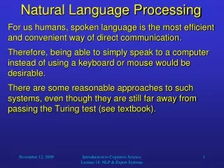
What’s Natural Language Processing? • Depends on your point of view • Psychology: Understand human language processing • How do we learn language? • How do we understand language? • How do we produce language? • How is language tied to thought? • Engineering: Build systems to process language • Build dialogue-based call centers • Build information retrieval engines • Build question-answering systems • Design general algorithms for a range of applications
NLP is Turing Test Hard • “Computer Machinery & Intelligence.” 1950. Alan Turing. • The Big Question I propose to consider the question, 'Can machines think?' • The Imitation Game The new form of the problem can be described' in terms of a game which we call the 'imitation game'. It is played with three people, a man (A), a woman (B), and an interrogator (C) who may be of either sex. The interrogator stays in a room apart from the other two. The object of the game for the interrogator is to determine which of the other two is the man and which is the woman. He knows them by labels X and Y, and at the end of the game he says either 'X is A and Y is B' or 'X is B and Y is A'. • Turing’s Test We now ask the question, 'What will happen when a machine takes the part of A in this game?' Will the interrogator decide wrongly as often when the game is played like this as he does when the game is played between a man and a woman? These questions replace our original, 'Can machines think?' Alan Turing
Brief History of NLP • 1950s: Machine Translation • Abandoned due to lack of computing resources • 1960s: Despair • Problem considered impossible philosophically (Quine) • Problem considered impossible linguistically (Chomsky) • 1970s: Dawn of Artificial Intelligence • “Full” dialog systems (eg. SHRDLU) • Symbolic processing in LISP • Early theories of semantics; first big systems (eg. LUNAR) • First information retrieval systems W.V.O. Quine
1970s Example: SHRDLU Terry Winograd. 1971. MIT Ph.D. Thesis. Person: PICK UP A BIG RED BLOCK. Computer: OK. (does it) Person: GRASP THE PYRAMID. Computer: I DON'T UNDERSTAND WHICH PYRAMID YOU MEAN. Person: FIND A BLOCK WHICH IS TALLER THAN THE ONE YOU ARE HOLDING AND PUT IT INTO THE BOX. Computer: BY "IT", I ASSUME YOU MEAN THE BLOCK WHICH IS TALLER THAN THE ONE I AM HOLDING. Computer: OK. (does it) Person: WHAT DOES THE BOX CONTAIN? Computer: THE BLUE PYRAMID AND THE BLUE BLOCK. Person: WHAT IS THE PYRAMID SUPPORTED BY? Computer: THE BOX. Person: HOW MANY BLOCKS ARE NOT IN THE BOX? Computer: FOUR OF THEM. Person: IS AT LEAST ONE OF THEM NARROWER THAN THE ONE WHICH I TOLD YOU TO PICK UP? Computer: YES, THE RED CUBE. Terry Winograd • This is one of the only dialogs it knows. • SHRDLU is too stupid • to make mistakes. • Beautiful “Demo-ware”
History of NLP (2) • 1980s: Rationalism • Focus on syntactic and semantic grammars and discourse • Logical frameworks for grammar (LFG, GPSG) and for knowledge (KL-ONE, CYC, etc.) • Everything hand-built • Couldn’t scale; wasn’t robust Ron Brachman (KL-ONE) Joan Bresnan (LFG) Gerald Gazdar (GPSG)
1980s Example: CYC • CYC’s way of saying “every animal has a mother” (forAll ?A (implies (isa ?A Animal) (thereExists ?M (and (mother ?A ?M) (isa ?M FemaleAnimal))))) • Couldn’t make all the world’s knowledge consistent • Maintenance is a huge nightmare • But it still exists and is getting popular again due to the “Semantic Web” in general and WordNet in NLP • Check out the latest at opencyc.org Doug Lenat
History of NLP (3) • 1990s and 2000s: Empiricism • Focus on simpler problems like part-of-speech tagging and simplified parsing (e.g. Penn TreeBank) • Focus on full coverage (earlier known as “robustness”) • Focus on Empirical Evaluation • Still symbolic! • Examples in the rest of the talk • The Future? • Applications? • Still waiting for our Galileo (not even Newton, much less Einstein)
Current Paradigm 1. Express a “problem” • Computer science sense of well-defined task • Analyses must be reproducible in order to test systems • This is the first linguistic consideration • Examples: • Assign parts of speech from a given set (noun, verb, adjective, etc.) to each word in a given text. • Find all names of people in a specified text. • Translate a given paragraph of text from Arabic to English • Summarize 100 documents drawn from a dozen newspapers • Segment a broadcast news show into topics • Find spelling errors in email messages • Predict most likely pronunciation for a sequence of characters
Current Paradigm (2) • Generate Gold Standard • Human annotated training & test data • Most precious commodity in the field • Tested for inter-annotator agreement • Do two annotators provide the same annotation? • Typically measured with kappa statistic • (P-E)/(1-E) • P: Proportion of cases for which annotators agree • E: Expected proportion of agreements [assuming random selection according to distribution] • Difficult for non-deterministic generation tasks • Eg. Summarization, translation, dialog, speech synthesis • System output typically ranked on an absolute or relative scale • Agreement requires ranking comparison statistics and correlations • Free in other cases, such as language modeling, where test data is just text.
Current Paradigm (3) 3. Build a System • Divide Training Data into Training and Tuning sets • Build a system and train it on training data • Tune it on tuning data 4. Evaluate the System • Test on fresh test data • Optional: Go to a conference to discuss approaches and results
Example Heuristic System: EngCG • EngCG is the most accurate English part-of-speech tagger: 99+% accurate • Try it online: http://www.lingsoft.fi/cgi-bin/engcg • Lexicon plus 4000 or so rules with a 700,000 word hand-annotated development corpus • Several person-years of skilled labor to compile the rule set • Example output: • The_DET • free_A • cat_N • prowls_Vpres • in_PREP • the_DET • woods_Npl • . Atro Voutilainen
Example Heuristic System: EngCG (2) • Consider example input “to Miss Sloan” • Lexically, from the dictionary, the system starts with: "<to>" "to" PREP "to" INFMARK "<*miss>" "miss" <*> <SVO> <SV> V INF "miss" <*> <Title> N NOM SG "<*sloan>" "sloan" <*> <Proper> N NOM SG • Grammatically, “Miss” could be an infinitive or a noun here (and “to” an infinitive marker or a preposition, respectively). However: • “miss” is written in the upper case, which is untypical for verbs • the word is followed by a proper noun, an extremely typical context for the titular noun “miss” Timo Järvinen
Example Heuristic System (EngCG 3) • Lexical Context: “to[PREP,INFMARK] Miss[V,N] Sloan[N]” • Rules work by narrowing or transforming non-determinism • The following rule can be proposed: SELECT ("miss" <*> N NOM SG) (1C (<*> NOM)) (NOT 1 PRON) ; • This rule selects the nominative singular reading of the noun “miss” written in the upper case (<*>) if the following word in a non-pronoun nominative written in the upper case (i.e. also abbreviations are accepted). • A run against the test corpus shows that the rule makes 80 correct predictions and no mispredictions. • This suggests that the collocational hypothesis was a good one, and the rule should be included in the grammar. • http://www.ling.helsinki.fi/~avoutila/cg/doc/
“Machine Learning” Approaches • “Learning” is typically of parameters in a statistical model. • Often not probabilistic • E.g. Vector-based information retrieval; support-vector machines • Statistical analysis is rare • E.g. Hypothesis testing, posterior parameter distribution analysis, etc. • Usually lots of data and not much known problem structure (weak priors in Bayesian sense) • Types of Machine Learning Systems • Classification: Assign input to category • Transduction: Assign categories to sequence of inputs • Structure Assignment: Determine relations
Simple Information Retrieval • Problem: Given a query and set of documents, classify each document as relevant or irrelevant to the query. • Query and document are both sequences of characters • May have some structure, which can also be used • Effectiveness Measures (against gold standard) • Precision • # correctly classfied as relevant / # classified as relevant • = True Positives / (True Positives + False Positives) • Recall • # correctly classified as relevant / # actually relevant • = True Positives / (True Positives + False Negatives) • F-measure • (Precision + Recall) / 2*Precision*Recall
TREC 2004 Ad Hoc Genomics Track • Documents = Medline Abstracts PMID- 15225994 DP - 2004 Jun TI - Factors influencing resistance of UV-irradiated DNA to the restriction endonuclease cleavage. AD - Institute of Biophysics, Academy of Sciences of the Czech Republic, Kralovopolska 135, CZ-612 65 Brno, Czech Republic. LA - eng PL - England SO - Int J Biol Macromol 2004 Jun;34(3):213-22. FAU - Kejnovsky, Eduard FAU - Kypr, Jaroslav AB - DNA molecules of pUC19, pBR322 and PhiX174 were irradiated by various doses of UV light and the irradiated molecules were cleaved by about two dozen type II restrictases. The irradiation generally blocked the cleavage in a dose-dependent way. In accordance with previous studies, the (A + T)-richness and the (PyPy) dimer content of the restriction site belongs among the factors that on average, cause an increase in the resistance of UV damaged DNA to the restrictase cleavage. However, we observed strong effects of UV irradiation even with (G + C)-rich and (PyPy)-poor sites. In addition, sequences flanking the restriction site influenced the protection in some cases (e.g. HindIII), but not in others (e.g. SalI), whereas neoschizomer couples SmaI and AvaI, or SacI and Ecl136II, cleaved the UV-irradiated DNA similarly. Hence the intrastrand thymine dimers located in the recognition site are not the only photoproduct blocking the restrictases. UV irradiation of the …
TREC (cont.) • Queries = Ad Hoc “Topics” <TOPIC> <ID>51</ID> <TITLE>pBR322 used as a gene vector</TITLE> <NEED>Find information about base sequences and restriction maps in plasmids that are used as gene vectors.</NEED> <CONTEXT>The researcher would like to manipulate the plasmid by removing a particular gene and needs the original base sequence or restriction map information of the plasmid.</CONTEXT> </TOPIC> • Task: Given 4.5 million documents (9 GB raw text) and 50 query topics, return 1000 ranked results per query • (I used Apache’s Jakarta Lucene for the indexing (it’s free), and it took about 5 hours; returning 50,000 results took about 12 minutes, all on my home PC. Scores are out in August or September before this year’s TREC conference.)
Vector-Based Information Retrieval • “Standard” Solution (Salton’s SMART; Jakarta Lucene) • Tokenize documents by dividing characters into “words” • Simple way to do this is at spaces or on punctuation characters • Represent a query or document as a word vector • Dimensions are words; values are frequencies • E.g. “John showed the plumber the sink.” • John:1 showed:1 the:2 plumber:1 sink:1 • Compare query word vectory Q with document word vector D • Angle between document and query • Roughly speaking, a normalized proportion of shared words • Cosine(Q,D) = SUMword Q(word) * D(word) / length(Q) / length(D) • Q(word) is word count in query Q; D(word) is count in document D • length(V) = SQRT( SUMword V(word) * V(word) ) • Return ordered results based on score • Documents above some threshold are classified as relevant • Fiddling weights is a cottage industry Gerard Salton
Trading Precision for Recall • Higher Threshold = Lower Recall & Higher Precision • Plot of values is called a “Received Operating Curve”
Other Applications of Vector Model • Spam Filtering • Documents: collection of spam; collection of non-spam • Query: new email • (I don’t know if anyone’s doing this this way; more on spam later) • Call Routing • Problem: Send customer to right department based on query • Documents: transcriptions of conversations for a call center location • Queries: Speech rec of customer utterances • See my and Jennifer Chu-Carroll’s Computational Linguistics article • One of few NLP dialog systems actually deployed • Also used for automatic answering of customer support questions (e.g. AOL Germany was using this approach)
Applications of Vector Model (cont.) • Word “Similarity” • Problem: Car~driver, beans~toast, duck~fly, etc. • Documents: Words found near a given word • Queries: Word • See latent-semantic indexing approach (Susan Dumais, et al.) • Coreference • 45 different “John Smith”s in 2 years of Wall St. Journal • E.g. Chairman of General Motors; boyfriend of Pocohantas • Documents: Words found near a given mention of “John Smith” • Queries: Words found near new entity • Word sense disambiguation problem very similar • See Baldwin and Bagga’s paper
The Noisy Channel Model • Shannon. 1948. A mathematical theory of communication. Bell System Technical Journal. • Seminal work in information theory • Entropy: H(p) = SUMx p(x) * log2 p(x) • Cross Entropy: H(p,q) = SUMx p(x) * log2 q(x) • Cross-entropy of model vs. reality determines compression • Best general compressors (PPM) are character-based language models; fastest are string models (Zip class), but 20% bigger on human language texts • Originally intended to model transmission of digital signals on phone lines and measure channel capacity. Claude Shannon
Noisy Channel Model (cont.) • E.g. x, x’ are sequence of words; y is seq of typed characters, possibly with typos, misspellings, etc. • Generator generates a message x according to P(x) • Message passes through a “noisy channel” according to P(y|x): probability of output signal given input message • Decoder reconstructs original message via Bayesian Inversion: • ARGMAXx’ P(x’|y) [Decoding Problem] • = ARGMAXx’ P(x’,y) / P(y) [Definition of Conditional Probability] • = ARGMAXx’ P(x’,y) [Denominator is Constant] • = ARGMAXx’ P(x’) * P(y|x’) [Definition of Joint Probability]
Speech Recognition • Almost all systems follow the Noisy Channel Model • Message: Sequence of Words • Signal: Sequence of Acoustic Spectra • 10ms Spectral Samples over 13 bins • Like a stereo sound level meters measured 100 times/second • Some Normalization • Decoding Problem: ARGMAXx’ P(words|sounds) = ARGMAXx’ P(words,sounds) / P(sounds) = ARGMAXx’ P(words,sounds) = ARGMAXx’ P(words) * P(sounds|words) • Language Model: P(words) = P(w1,…,wN) • Acoustic Model: P(sounds|words) = P(s1,…,sM|w1,…,wN) Stereo Level Meter
Spelling Correction • Application of Noisy Channel Model • Problem: Find most likely word given spelling ARGMAXWord P(Word|Spelling) = ARGMAXWord P(Spelling|Word) * P(Word) • Example: • “the” = ARGMAXWord P(Word| “hte”) because P(“the”) * P(“hte”| “the”) > P(“hte”) * P(“hte”| “hte”) • Best model of P(Spelling|Word) is a mixture of: • Typing “mistake” model • Based on common typing mistakes (keys near each other) • substitution, deletion, insertion, transposition • Spelling “mistake” model • English ‘f’ likely for ‘ph’, ‘i’ for ‘e’, etc.
Transliteration & Gene Homology • Transliteration like spelling with two different languages • Best models are paired transducers: • P(pronuncation | spelling in language 1) • P(spelling in language 2 | pronunciation) • Languages may not even share character sets • Pronunciations tend to be in IPA: International Phonetic Alphabet • Sounds only in one language may need to be mapped to find spellings or pronunciations • Applied to Arabic, Japanese, Chinese, etc. • See Kevin Knight’s papers • Can also be used to find abbreviations • Very similar to gene similarity and alignment • Spelling Model replaced by mutation model • Works over protein sequences Kevin Knight
Chinese Tokens & Arabic Vowels • Chinese is written without spaces between tokens • “Noise” in coding is removal of spaces: • Characters + Dividers Characters • Decoder finds most likely original dividers: • Characters Characters + Dividers • ARGMAXVowels P(Characters | Characters+Dividers) * P(Characters+Dividers) = ARGMAXVowels P(Characters+Dividers) • Arabic is written without vowels • “Noise”/Coding is removal of vowels • Consonants + Vowels Consonants • Decode most likely original sequence: • Consonants Consonants + Vowels • ARGMAXVowels P(Consonants|Consonants+Vowels) * P(Consonants+Vowels) = ARGMAXVowels P(Consonants+Vowels)
N-gram Language Models • P(word1,…,wordN) = P(word1) [Chain Rule] * P(word2 | word1) * P(word3 | word2, word1) * … * P(wordN | wordN-1,wordN-2, …, word1) • N-gram approximation = N-1 words of context: P(wordK | wordK-1,wordK-2, …, word1) ~ P(wordK | wordK-1,wordK-2, …, wordK-N+1) • E.g. trigrams: P(wordK | wordK-1,wordK-2, …, word1) ~ P(wordK | wordK-1,wordK-2) • For commercial speech recognizers, usually bigrams (2-grams). • For research recognizers, the sky’s the limit (> 10 grams)
Smoothing Models • Maximum Likelihood Model • PML(word | word-1, word-2) = Count(word-2, word-1, word) / Count(word-2, word-1) • Count(words) = # of times sequence appeared in training data • Problem: If Count(words) is 0, then estimate for word is 0, and estimate for whole sequence is 0. • If Count(words) = 0 in denominator, choose shorter context • But real likelihood is greater than 0, even if not seen in training data. • Solution: Smoothe maximum likelihood model
Linear Interpolation • “Backoff” via Linear Interpolation: P’(w| w1,…,wK) = lambda(w1,…,wK) * PML(w| w1,…,wK) + (1-lambda(w1,…,wK)) * P’(w| w1,…,wK-1) P’(w) = lambda() * PML(w) + (1-lambda() * U) U = uniform estimate = 1/possible # outcomes • Witten-Bell Linear Interpolation lambda(words) = count(words) / ( count(words) + K * numOutcomes(words) ) K is a constant that is typically tuned (usually ~ 4.0)
Character Unigram Language Model • May be familiar from Huffman coding • Assume 256 Latin1 characters; uniform U = 1/256 • “abracadabra” counts a:5 b:2 c:1 d:1 r:2 • P’(a) = lambda() * PML(a) + (1-lambda() * U) = (11/31 * 5/11) + (1-11/31)*1/256 ~ 1/6 + 1/750 PML(a) = count(a) / count() = 5/11 lambda() = count() / (count() + 4 * outcomes()) = 11 / (11 + 4*5) = 11/31 • P’(z) = (1-lambda()) * U = 11/31 * 1/256 ~ 1/750
Compression with Language Models • Shannon connected coding and compression • Arithmetic Coders code a symbol using log2 P(symbol|previous symbols) bits [details are too complex for this talk; basis for JPG] • Arithmetic Coding codes below the bit level • A stream can be compressed by dynamically predicting likelihood of next symbol given previous symbols • Built language model based on previous symbols • Using a character-based n-gram language model for English using Witten-Bell smoothing, the result is about 2.0 bits/character. • Best compression is using unbounded length contexts. • See my open-source Java implementation: www.colloquial.com/ArithmeticCoding/ • Best model for English text is around 1.75 bits/character; it involves a word model and punctuation model and has only been tested on a limited corpus (Brown corpus) [Brown et al. (IBM) Comp Ling paper]
Classification by Language Model • The usual Bayesian inversion: ARGMAXCategory P(Category | Words) = ARGMAXCategory P(Words|Category) * P(Category) • Prior Category Distribution P(Category) • Language Model per Category P(Words|Category) = PCategory(Words) • Spam Filtering • P(SPAM) is proportion of input that’s spam • PSPAM(Words) is spam language model (E.g. P(Viagra) high) • PNONSPAM(Words) is good email model (E.g. P(HMM) high) • Author/Genre/Topic Identification • Language Identification
Hybrid Language Model Applications • Very often used for rescoring with generation • Generation • Step 1: Select topics to include with clauses, etc. • Step 2: Search with language model for best presentation • Machine Translation • Step 1: Symbolic translation system generates several alternatives • Step 2: One with highest langauge model score is selected • See Kevin Knight’s papers
Information Retrieval via Language Models • Each document generates a language model PDoc • Smoothing is critical and can be against background corpus • Given a query Q consisting of words w1,…,wN • Calculate ARGMAXDoc PDoc(Q) • Beats simple vector model because it handles dependencies; not just simple bag of words • Often vector model is used to restrict collection to a subset before rescoring with language models • Provides way to incorporate prior probability of documents in a sensible way • Does not directly model relevance • See Zhai and Lafferty’s paper (Carnegie Mellon)
HMM Tagging Models • A tagging model attempts to classify each input token • A very simple model is based on a Hidden Markov Model • Tags are the “hidden structure” here • Reduce Conditional to Joint and invert as before: • ARGMAXTags P(Tags|Words) = ARGMAX P(Tags) * P(Words|Tags) • Use bigram model for Tags [Markov assumption] • Use smoothed one-word-at-a-time word approximation: • P(w1,…,wN | t1, …, tN) ~ PRODUCT1<=k<=N P(wk | tk) • P(w|t) = lambda(t) * PML(w) + (1-lambda(t)) UniformEstimate • Measured by Precision and Recall and F score • Evaluations often include partial credit (reader beware)
Penn TreeBank Part-of-Speech Tags • Example sentence with tags: Battle-tested/JJ Japanese/JJ industrial/JJ managers/NNS here/RB always/RB buck/VBP up/RP nervous/JJ newcomers/NNS with/IN the/DT tale/NN of/IN the/DT first/JJ of/IN their/PP$ countrymen/NNS to/TO visit/VB Mexico/NNP ,/, a/DT boatload/NN of/IN samurai/FW warriors/NNS blown/VBN ashore/RB 375/CD years/NNS ago/RB ./. • Tokenization of “battle-tested” is tricky here • Description of Tags • JJ: adjective, RB: adverb, NNS: plural noun, DT: determiner, VBP: verb, IN: preposition, PP$: possessive, NNP: proper noun, VBN: participail verb, CD: numberal • Annotators disagree on 3% of the cases • Arguably this is because the tagset is ambiguous – bad linguistics, not impossible problem • Best Treebank Systems are 97% accurate (about as good as humans)
Pronunciation & Spelling Models • Phonemes: sounds of a language (42 or so in English) • Graphemes: letters of a language (26 in English) • Many-to-many relation • e [] [Silent ‘e’] • e IY [Long ‘e’] • t+h TH [TH is one phoneme] o+u+g+h OO [“through”] • x K+S • Languages vary wildly in pronunciation entropy (ambiguity) • English is highly irregular; Spanish is much more regular • Pronunciation model • P(Phonemes|Graphemes) • Each grapheme (letter) is transduced as 0, 1, or 2 phonemes • “ough” OO via o[OO], u [], g[], h[] • Can also map multiple symbols • Spelling Model just reverses pronunciation model • See Alan Black and Kevin Lenzo’s papers
Named Entity Extraction • CoNLL = Conference on Natural Language Learning • Tagging names of people, locations and organizations Wolff B-PER , O currently O a O journalist O in O Argentina B-LOC , O played O with O Del B-PER Bosque I-PER in O • O is out of name, B-PER is begin person name, I-PER continues person name, etc. • “Wolff” is person, “Argentina” location and “Del Bosque” a person
Entity Detection Accuracy • Message Understanding Conference (MUC) Partial Credit • ½ score for wrong boundaries, right tag • ½ score for right bounaries, wrong tag • English Newswire: People, Location, Organization • 97% precision/recall with partial credit • 90% with exact scoring • English Biomedical Literature: Gene • 85% with partial credit; 70% without • English Biomedical Literature: Precise Genomics • GENIA corpus (U. Tokyo): 42 categories including proteins, DNA, RNA (families, groups, substructures), chemicals, cells, organisms, etc. • 80% with partial credit • 60% with exact scoring • See our LingPipe open-source software: www.aliasi.com/lingpipe
CoNLL Phrase Chunks (+POS, +Entity) • Find Noun Phrase, Verb Phrase and PP chunks: U.N. NNP I-NP I-ORG official NN I-NP O Ekeus NNP I-NP I-PER heads VBZ I-VP O for IN I-PP O Baghdad NNP I-NP I-LOC . . O O • First column contains tokens • Second column contains part of speech tags • Third column contains phrase chunk tags • Fourth column contains entity chunk tags • Shallow parsing as “chunking” originated by Ken Church Ken Church
2003 BioCreative Evaluation • Find gene names in text • Simple one category problem • Training data in form @@98823379047 Varicella-zoster/NEWGENE virus/NEWGENE (/NEWGENE VZV/NEWGENE )/NEWGENE glycoprotein/NEWGENE gI/NEWGENE is/OUT a/OUT type/NEWGENE 1/NEWGENE transmembrane/NEWGENE glycoprotein/NEWGENE which/OUT is/OUT one/OUT component/OUT of/OUT the/OUT heterodimeric/OUT gE/NEWGENE :/OUT gI/NEWGENE Fc/NEWGENE receptor/NEWGENE complex/OUT ./OUT • In reality, we spend a lot of time munging oddball data formats. • And like this example, there are lots of errors in the training data. • And it’s not even clear what’s a “gene” in reality. Only 75% kappa inter-annotator agreement on this task.
Viterbi Lattice-Based Decoding • Work left-to-right through input tokens • Node represents best analysis ending in tag (Viterbi = best path) • Back pointer is to history; when done, backtrace outputs best path • Score is sum of token joint log estimates: • log P(token|tag) + log P(tag|tag-1)
Sample N-best Output • First 7 outputs for “Prices rose sharply today” • Rank. Log Prob : Tag/Token(s) 0. -35.612683136497516 : NNS/prices VBD/rose RB/sharply NN/today 1. -37.035496392922575 : NNS/prices VBD/rose RB/sharply NNP/today 2. -40.439580756197934 : NNS/prices VBP/rose RB/sharply NN/today 3. -41.86239401262299 : NNS/prices VBP/rose RB/sharply NNP/today 4. -43.45450487625557 : NN/prices VBD/rose RB/sharply NN/today 5. -44.87731813268063 : NN/prices VBD/rose RB/sharply NNP/today 6. -45.70597331609037 : NNS/prices NN/rose RB/sharply NN/today • Likelihood for given subsequence with tags is sum of all estimates for sequences containing that subsequence • E.g. P(VBD/rose RB/sharply) is the sum of probabilities of 0, 1, 4, 5, …
Forward/Backward Algorithm: Confidence • Viterbi stores best-path score at node • Assume all paths complete; sum of all outgoing arcs 1.0 • Forward stores sum of all paths to node from start • Total probability that node is part of answer • Normalized so all paths complete; all outgoing paths sum to 1.0 • Backward stores sum of all paths from node to end • Also total probability that node is part of answer • Also normalized in same way • Given a path P, its total likelihood is product of: • Forward score to start of path (likelihood of getting to start) • Backward score from end of path (likelihood of finishing from end = 1.0) • Score of arcs along the path itself • This provides confidence of output, e.g. that “John Smith” is a person in “Does that John Smith live in Washington?” or that “c-Jun” is a gene in “MEKK1-mediated c-Jun activation”
Viterbi Decoding (cont.) • Basic decoder has asymptotic complexity O(n*m2) where n is the number of input symbols and m is the number of tags. • Quadratic in tags because each slot must consider each previous slot • Memory can be reduced to the number of tags if backpointers are not needed • Keeping n-best at nodes increases time and memory requirements by n • More history requires more states • Bigrams, states = tags • Trigrams, states = pairs of tags • Pruning removes states • Remove relatively low-scoring paths Andrew J. Viterbi
Common Tagging Model Features • More features usually means better systems if features’ contributions can be estimated • Previous/Following Tokens • Previous/Following Tags • Token character substrings (esp for biomedical terms) • Token prefixes or suffixes (for inflection) • Membership of token in dictionary or gazetteer • Shape of token (capitalized, mixed case, alphanumeric, numeric, all caps, etc.) • Long range tokens (trigger model = token appears before) • Vectors of previous tokens (latent semantic indexing) • Part-of-speech assignment • Dependent elements (who did what to whom)
Adaptation and Corpus Analysis • Can retrain based on output of a run • Known as “adaptation” of a model • Common for language models in speech dictation systems • Amounts to “semi-supervised learning” • Original training corpus is supervised • New data is just adapted by training on high-confidence analyses • Can look at whole corpus of inputs • If a phrase is labeled as a person somewhere, it can be labeled elsewhere – context may cause inconsistencies in labeling • Can find common abbreviations in text and know they don’t end sentences when followed by periods
Who did What to Whom? • Previous examples involved so-called “shallow” analyses • Syntax is really about who did what to whom (when, why, how, etc.) • Often represented via dependency relations between lexical items; sometimes structured