Download
1 / 49
500 likes | 711 Views
Theoretical distributions Lorenz Wernisch. Distributions as compact data descriptions. List of numbers becomes organized in a histogram distribution captures statistical essentials. 66 2463 933 1287 297 777 1431 954 588 567 714 591. Gamma function with l = 2.660301

E N D
Distributions as compact data descriptions List of numbers becomes organized in a histogram distribution captures statistical essentials • 66 • 2463 • 933 • 1287 • 297 • 777 • 1431 • 954 • 588 • 567 • 714 • 591 • ..... Gamma function with l = 2.660301 s = 358.4419
A scoring scheme • Compare a new target (keyword, DNA sequence) • with objects (HTML pages, known DNA sequences) • in a database to find matching objects. • Each comparison results in a score database scores comparison -46 target -42 -59 -45 330 -53
Compare target score with rest of scores The scores of unrelated (random) database hits number Score 330 lies here, way outside the heap of random scores scores
Fit a Normal (Gaussian) distribution m = -47.1 score s = 330 s = 20.8
Probability for high scores The red area is the probability that a random N(-47.1,20.8) distributed variable has score > 0 Pr[s > 0] = 0.0117
Objectives • At the end of the day you should be able to • do some combinatorial counting • mention one typical example for each of the following distributions: Binomial, Poisson, Normal, Chi-square, t, Gamma, Extreme Value • plot these distributions in R • fit one of the above distributions to a set of discrete or continuous data using maximum likelihood estimates in R
How many ways are there to order numbers • 3 numbers? 123, 213, ... • 4 numbers using the result for 3 numbers? • n numbers using the result for (n-1) numbers?
The subsets of size k in a set of size n 8 10 • How many subsets of k = 3 • in set of n = 10 elements? • Idea: • enumerate all orderings • take first three • ....... • 3 7 5 1 10 9 4 2 3 8 • 3 5 7 1 10 9 4 2 3 8 • 5 7 3 9 4 3 1 10 8 2 • ....... 9 5 3 4 7 1 2 6 How many orderings give the same result?
Binomial coefficient • Number of choosing subsets of k from set of n • “n choose k” • Alternative form:
Very simple: the Bernoulli distribution • A coin with two sides, side 0 (tail) and side 1 (head), • has been tested with thousands of throws: • 60% gives 0 40% gives 1 • P[0] = 0.6 P[1] = 0.4 • The coin is a Bernoulli variable X with p = 0.4 • expectation • variance
Flipping a coin • What is the probability of the following runs? • P[0 1 0 1 1 0 0 0 1 0] = • P[1 1 0 0 0 0 1 0 0 1] = • P[0 0 0 1 1 1 0 1 0 0] = • How many of such runs with four 1s exist? • What is the total probability of four 1s in 10 throws?
Binomial distribution 1 Experiment: 100 coin tosses with p = Pr[side 1] = 0.4: expecting about 40 1s (but not exactly 40) 1000 experiments: (1000 x 100 coin tosses) number of experiments out of 1000 number of 1s out of 100
R program for binomial plot • # generate 1000 simulations • x <- rbinom(1000,100,0.4) • # generate vector from 20 to 60 • z <- 20:60 • # plot the histogram from 20 to 60 • # with no labels • hist(x,breaks=z,xlab="",ylab="",main="", • xlim=c(20,60)) • # draw points of binomial distribution • # for 1000 experiments, line width 2 • lines(z,1000*dbinom(z,100,0.4), • type="p",lwd=2)
Binomial distribution p = 0.82 • Cumulative distribution • function (cdf) • probability density • function (pdf) binomial n = 100 p = 0.4 l = 44
R functions for distributions • Each distribution comes with a set of R functions. • Binomial distribution with parameters • n = size, p = prob • probability density function, pdf • dbinom(x,size,prob) • cumulative distribution function, cdf • pbinom(x,size,prob) • generate random examples • rbinom(number,size,prob) • More information: help(dbinom)
R program for two binomial plots • # make space for two plots • par(mfrow=c(2,1)) • z <- 20:60 • # cdf first, “s” for cdf plot • plot(z,pbinom(z,100,0.4),type="s") • # pdf next, “h” for vertical lines • plot(z,dbinom(z,100,0.4),type="h") • # add some points, “p” for points • lines(z,dbinom(z,100,0.4),type="p") • # one plot only in future • par(mfrow=c(1,1))
Binomial for large n and small p • Number n of throws very large • Tiny probability p for throwing a 1 • Expected number of 1s constant: l = np n = 50 p = 0.06 l = 3 0 1 n = 100 p = 0.03 l = 3 0 1
Poisson distribution • If, on average, one sees l heads between 0 and 1 what is the probability of seeing k heads? • Make grid between 0 and 1 finer and finer, keeping l = np constant: • For example: requires some calculation with limit
Poisson distribution • cdf • pdf • expectation • variance • ppois(x,lambda) • dpois(x,lambda) • rpois(n,x,lambda) Poisson l = 2.7
Application of Poisson: database search • Query sequence against database of • “random” (that is, nonrelated) sequences: • p = Pr[database sequence looks significant, hit] • n = number of sequences in database • n is large and p is small, “E-value” l = np • Chance to get at least one wrong (random) hit:
Normal distribution N(m,s) P[X<7] = 0.841 Cumulative distribution function: Normal m = 5, s = 2 Probability density function: Expectation Variance
R program for two normal plots of N(5,2) • par(mfrow=c(2,1)) • z <- seq(-2,12,0.01) • plot(z,pnorm(z,5,2),type="l",frame.plot=F, • xlab="",ylab="",lwd=2) • plot(z,dnorm(z,5,2),type="l",frame.plot=F, • xlab="",ylab="",lwd=2) • # plot the hashing of the pdf • z <- seq(-2,7,0.1) • lines(z,dnorm(z,5,2),type="h") • par(mfrow=c(1,1))
Normal distribution as limit of Binomial • increase n • constant p • Binomial • Normal • (less and less • skewed)
Central limit theorem • Independent random variables Xi all with the same distribution X: E[X] = m and V[X] = s 2 • The sum • is normal N(0,1) in the limit: • or equivalently: density
Fitting a distribution • 200 data points in histogram • seem to come from • normal distribution • To fit a normal distribution • N(m,s), we need to know • two parameters: m and s • How to find them?
Maximum likelihood estimators (MLE) • Density function f(x; m,s) • Sample x = {x1, x2, ..., xn} from pdf f(x; m,s) • Likelihood for fixed sample depends on parameters m and s • Log-likelihood • We now try to find the m and s that maximize the • likelihood or log-likelihood
MLE for normal distribution is simple • For normal distribution the MLE of m and s is • straightforward: it’s just the mean and standard • deviation of the data: • # stepsize stsz of histogram, datavector x • z <- seq(min(x)-stsz,max(x)+stsz,0.01) • lines(z, • length(x)*stsz*dnorm(z,mean(x),sd(x)) )
Fitting a distribution by MLE in R • Data points xi: x <- scan(“numbers.dat”) • For each data point xi a density value f(xi; m,s) • We are looking for m and s that make all these density values as large as possible together • Parameters m and s should maximize • sum(log(dens(x,mu,sigma))) • or minimize -sum(log(dens(x,mu,sigma)))
MLE for normal distribution in R • # define the function to minimize • # it takes a vector p of 2 parameters • f.neglog <- function(p) • -sum(log(dnorm(x,p[1],p[2]))) • # starting values for the 2 parameters • start.params <- c(0,1) • # minimize the target function • mle.fit <- nlm(f.neglog,start.params) • # get the estimates for the parameters • mle.fit$estimate
Points to notice about MLE in R • The nlm algorithm is an iterative heuristic minimization algorithm and can fail! • Choice of the right starting values for the parameters is crucial: an initial guess from the histogram can help • For location and scale parameters mean(x) and sd(x) is often a good guess • Check the result by fitting the density function with the calculated parameters to the histogram
Exponential distributionExp(l) • cdf • pdf • Expectation • Variance • pexp(x,lambda) • dexp(x,lambda) • rexp(n,x,lambda) Exponential l = 4
Exponential distribution and Poisson process • The exponential distribution as limiting process, tiny probability p, many trials n for throwing a 1 in the unit interval [0,1]: l = np • How long does it take until the first 1? • 18.1% chance of seeing a 1 in the indicated region 0 1
MLE estimate for exponential function • Maximum likelihood estimate for l in • 1) • 2) • 3) l =
The Gamma function • is the continuation of the factorial n! to real numbers: • and is used in many distribution functions • Moreover,
Gamma distribution • density function, pdf: • expectation • variance • pgamma(x,alpha,lambda) • dgamma(x,alpha,lambda) • rgamma(n,x,alpha,lambda) Gamma a = 3, l = 4
a = 1 a = 1/3 a = 3 a = 1/5 a = 5 Shape parameter of Gamma distribution
Gamma distribution and Poisson process • The gamma distribution as limiting process: tiny probability p, many trials n for throwing a 1 in the unit interval [0,1]: l = np • How long does it take until the third 1? • 0.11% chance of seeing three 1s in the indicated region 0 1
Example: waiting times in a queue • Time to service a person at the desk: • exponential with le = 1/(average waiting time) • If there are n persons in front of you, how is the time you have to wait distributed? • It turns out: the sum of n exponentially distributed • variables (waiting time for each person) is • Gamma distributed with a = n and l = le
Extreme value distribution • cumulative distribution cdf • probability density pdf • No simple form for • expectation and variance Extreme Value m = 3, s = 4
Examples for Extreme Value Distribution EVD • 1) An example from meteorology: • Wind speed is measured daily at noon: • Normal distribution around average wind speed • Monthly maximum wind speed is recorded as well • The monthly maximum wind speed does not follow a normal distribution, it follows an EVD • 2) Scores of sequence alignments (local alignments) often follow an EVD
R code for Extreme Value distribution • No predefined procedures for the EVD in R • Replace for example: • pexval <- function(x,mu=0,sigma=1) • exp(-exp(-(x-mu)/sigma)) • dexval <- function(x,mu=0,sigma=1) • 1/sigma*exp((x-mu)/sigma) • *pexval(x,mu,sigma) • pexval(x,3,4) • dexval(x,3,4)
c2 distribution • Standard normal random variables Xi, Xi~N(0,1), • The variable • has a cn2 distribution with n degrees of freedom • density • expectation • variance squared! pchisq(x,n) dchisq(x,n) rchisq(num,x,n)
n = 1 n = 2 n = 4 n = 6 n = 10 Shape of c2 distribution is actually Gamma function with a = n/2 and l = 1/2
t distribution • Z ~ N(0,1) independent of U ~ cn2 • then • has a t distribution with n degrees of freedom • density pt(x,n) dt(x,n) rt(num,x,n)
Shape of t distribution n = 10 N(0,1) • Approaches • normal N(0,1) • distribution • for large n • (n > 20 or 30) n = 3 n = 5 n = 1
Fitting chi-squared ort distribution w • Need location parameter • m and scale parameter s • the new density is • mu <- 3 • sig <- 2 • 1/sig*dt((x-mu)/sig),3) t with n = 3 m sw m = 3 s = 2
MLE for t distribution • # function to minimize with 3 parameters • # p[1] is m, p[2] is s, p[3] is n • f.neglog <- function(p) • -sum(log(1/p[2]*dt((x-p[1])/p[2],p[3]))) • # starting values for the 2 parameters • start.params <- c(0,1,1) • # minimize the target function • mle.fit <- nlm(f.neglog,start.params) • # get the estimates for the parameters • mle.fit$estimate