Download
1 / 65
750 likes | 1.14k Views
Chapter 8 Introduction to Turing Machines. Rothenberg, Germany. Outline. Problems that Computers Cannot Solve The Turing Machine (TM) Programming Techniques for TM’s Extensions to the Basic TM Restricted TM’s TM’s and Computers. 8.0 Introduction. Concepts to be taught ---

E N D
Chapter 8 Introduction to Turing Machines Rothenberg, Germany
Outline • Problems that Computers Cannot Solve • The Turing Machine (TM) • Programming Techniques for TM’s • Extensions to the Basic TM • Restricted TM’s • TM’s and Computers
8.0 Introduction • Concepts to be taught --- • Studying questions about what languages can be defined be any computational device?? • There are specific problems that cannot be solved by computers! --- undecidable! • Studying the Turing machine which seems simple, but can be recognized as an accurate model for what any physical computing device is capable of doing.
8.1 Problems That Computers Cannot Solve • Purpose of this section --- to provide an informal proof , C-programming-based introduction to proof of a specific problem that computers cannot solve. • The problem: whether the first thing a C program prints is hello, world. • We will give the intuition behind the formal proof.
8.1 Problems That Computers Cannot Solve • 8.1.1 Programs that print “Hello, World” • A C program that prints “Hello, World” : main() { print(“hello, world\n”); } • Define hello, world problemto be: determine whether a given C program, with a given input, prints hello, world as the first 12 characters that it prints.
8.1 Problems That Computers Cannot Solve • 8.1.1 Programs that print “Hello, World” • The problem described alternatively using symbols: Is there a programH that could examine any program P and input I for P, and tell whether P, run with I as its input, would print hello, world?(A programH means an algorithm in concept here.) • The answer is: undecidable! That is, there exists no such program H. We will prove this by contradiction.
I Hello-world tester H yes if P, with input I, prints“hello world” no if not. P Figure 8.3 8.1 Problems That Computers Cannot Solve • 8.1.2 Hypothetical “Hello, World” Tester • 1st step: assume H exists in the following form: • 2nd step: transform H to another form H2 in simple ways which can be done by C programs • 3rd step: prove H2 not existing. So H also not existing.
Figure 8.5 yes Hello-world tester H2 P hello, world 8.1 Problems That Computers Cannot Solve • 8.1.2 Hypothetical “Hello, World” Tester • 2nd step: • (1) transform H to H1 in the following way - • (2) transform H1to H2in the following way – Use P both as input and program! I yes Hello-world tester H1 Figure 8.4 hello, world (print ‘hello, world’ instead of ‘no’) P
Figure 8.5 yes Hello-world tester H2 P hello, world 8.1 Problems That Computers Cannot Solve • 8.1.2 Hypothetical “Hello, World” Tester • 2nd step (cont’d): • The function of H2 is: given any program P as input, if P prints hello world as first output, then H2makes output yes; if P does not prints hello world as first output, then H2 prints hello world.
Figure 8.6 yes Hello-world tester H2 H2 hello, world 8.1 Problems That Computers Cannot Solve • 8.1.2 Hypothetical “Hello, World” Tester • 3rd step: • Prove H2 does not exist as follows – • Let P for H2 in Fig. 8.5 (last figure) be H2itself, as follows: (H2 Takes H2 as input to itself)
Figure 8.6 yes Hello-world tester H2 H2 hello, world 8.1 Problems That Computers Cannot Solve • 8.1.2 Hypothetical “Hello, World” Tester • 3rd step (cont’d): • Prove H2 does not exist by contradiction as follows (cont’d) – • Now, (1) if the boxH2, given itself as input, makes outputyes, then it means that the input H2, given itself as input, prints hello world as first output. But this is contradictory because we just suppose that H2, given itself as input, makes outputyes.
Figure 8.6 yes Hello-world tester H2 H2 Hello, world 8.1 Problems That Computers Cannot Solve • 8.1.2 Hypothetical “Hello, World” Tester • 3rd step (cont’d): • Prove H2 does not exist as follows (cont’d) – • The above contradiction means the other alternative must be true (since it must be one or the other), that is --- (2) the boxH2, given itself as input, printshello, world. This then means that such H2, when taken as input H2to the boxH2(itself), will make the boxH2to make outputyes. Contradiction again because we just say that the boxH2, given itself as input, printshello, world.
Figure 8.6 yes Hello-world tester H2 H2 Hello, world 8.1 Problems That Computers Cannot Solve • 8.1.2 Hypothetical “Hello, World” Tester • 3rd step (cont’d): • Prove H2 does not exist as follows (cont’d) – • Since both cases lead to contradiction, we conclude that the assumption that H2 exists is wrong by the principle of contradiction for proof.
8.1 Problems That Computers Cannot Solve • 8.1.2 Hypothetical “Hello, World” Tester • 3rd step (cont’d): • H2 does not exist H1 does not exist (otherwise, H2 must exist) H does not exist (otherwise, H1 must exist) • The above self-contradiction technique, similar to the diagonalization technique (to be introduced later), was used by Alan Turing for proving undecidable problems.
8.1 Problems That Computers Cannot Solve • 8.1.3 Reducing One Problem to Another • Now we have an undecidable problem, which can be used to prove other undecidable problems by a technique of “problem reduction.” • That is, if we know P1 is undecidable, then we may reduce P1 to a new problem P2, so that we may prove P2 undecidable by contradiction in the following way: • If P2 is decidable, then P1 is decidable. • But P1 is known undecidable. So, contradiction! • Consequently, P2 is undecidable.
Construct P2 instance P1 instance yes Decide Old problem New problem no 8.1 Problems That Computers Cannot Solve • 8.1.3 Reducing One Problem to Another • An illustration of this idea is: if and only if
8.1 Problems That Computers Cannot Solve • 8.1.3 Reducing One Problem to Another • Example 8.1 We want to prove a new problem P2 (called calls-foo problem): “does program Q, given input y, ever call function foo?” to be undecidable. Solution: regard Q as P1; reduce P1: the hello-world problem to P2: the calls-foo problem in the following way: (continued in the next page)
8.1 Problems That Computers Cannot Solve • 8.1.3 Reducing One Problem to Another • Example 8.1 (cont’d) Solution: reduce P1 to P2 in the following way: • If Q has a function called foo, renameit and all calls to that function a new program Q1 doing the same as Q. (去除碰巧同名) • Add to Q1 a function foo doing nothing & not called a new Q2 • Modify Q2to remember the first 12 characters that it prints, storing them in a global array AQ3 • Modify Q3 so that whenever it executes any output statement, it checks A to see if it has written 12 characters or more, and if so, whether hello, world are the first characters. In that case, call the new function fooR with input z = y.
8.1 Problems That Computers Cannot Solve • 8.1.3 Reducing One Problem to Another • Example 8.1 (cont’d) Solution (cont’d): Now, (1) if Q with input y prints hello, world as its first output, then R will call foo; (2) if Q with input y does not print hello, world, then R will never call foo. (3) That is, R, with input z =y, calls fooif and only ifQ, with input y, prints hello, world. (4) So, if we can decide whether R, with input z, calls foo, then we can decide whether Q, with input y, prints hello, world. (5) But the latter is impossible, so the former is impossible.
Construct P2 instance P1 instance yes Decide no 8.1 Problems That Computers Cannot Solve • 8.1.3 Reducing One Problem to Another • The above example illustrates how to reduce a problem to another. • An illustration of this idea is: if and only if Old problem New problem
8.2 The Turing Machine • Concepts to be taught: • The study of decidability provides guidance to programmers about what they might or might not be able to accomplish through programming. • Previous problems are dealt with programs. But not all problems can be solved by programs.
8.2 The Turing Machine • Concepts to be taught: • We need a simple model to deal with other decision problems (like grammar ambiguity problems) • The Turing machine is one of such models, whose configuration is easy to describe, but whose function is the most versatile: all computations done by a modern computer can be done by a Turing machine. (a hypothesis!)
8.2 The Turing Machine • 8.2.1 The Quest to Decide All Mathematical Questions • At the turn of 20th century, D. Hilbert asked: “whether it was possible to find an algorithm for determining the truth or falsehood of any mathematical proposition.” (in particular, he asked if there was a way to decide whether any formula in the 1st-order predicate calculus, applied to integer, was true)
8.2 The Turing Machine • 8.2.1 The Quest to Decide All Mathematical Questions • In 1931, K. Gödel published his incompleteness theorem: “A certain formula in the predicate calculus applied to integers could notbe neither proved nor disproved within the predicate calculus.” • The proof technique is diagonalization, resembling the self-contradiction technique used previously.
8.2 The Turing Machine • 8.2.1 The Quest to Decide All Mathematical Questions • Natures of computational model --- • Predicate calculus --- declarative • Partial-recursive functions --- computational (a programming-language-like notion) • Turing machine --- computational (computer-like) (invented by Alan Turing several years before true computers were invented)
8.2 The Turing Machine • 8.2.1 The Quest to Decide All Mathematical Questions • Equivalence of maximal computational model: They all compute the same functions or recognize the same languages, having the same power of computation.
8.2 The Turing Machine • 8.2.1 The Quest to Decide All Mathematical Questions • Unprovable Church-Turing hypothesis (or thesis): Any general way to compute will allow us to compute only the partial-recursive functions (or equivalently, what the Turing machine or modern-day computers can compute).
Finitecontrol … … Xi X2 Xn X1 B B B B 8.2 The Turing Machine • 8.2.2 Notion for the Turing Machine • A model for Turing machine:
8.2 The Turing Machine • 8.2.2 Notion for the Turing Machine • A move of Turing machine includes: • change state; • write a tape symbol in the cell scanned; • move the tape head left or right. • Formal definition: A Turing machine (TM) is a 7-tuple M = (Q, S, G, d, q0, B, F) where • Q: a finite set of states of the finite control; • S: a finite set of input symbols; • G: a set of tape symbols, with S being a subset ofit;
8.2 The Turing Machine • 8.2.2 Notion for the Turing Machine • Formal definition (cont’d): • d: a transition function d(q, X) = (p, Y, D) where • q: the current state, in Q; • X: a tape symbol being scanned; • p: the next state, in Q; • Y: the tape symbol written on the cell being scanned, used to replace X; • D: either L (left) or R (right) telling the move direction of the tape head;
8.2 The Turing Machine • 8.2.2 Notion for the Turing Machine • Formal definition (cont’d): • q0: the start state, in Q; • B: the blank symbol in G,not in S (should not be an input symbol); • F: the set of final (or accepting) states. • A TM is a deterministic automaton with a two- way infinite tape which can be read and written in either direction.
8.2 The Turing Machine • 8.2.3 Instantaneous Descriptions for Turing Machine • The instantaneous description (ID) of a TM is represented by • X1X2…Xi1qXiXi+1…Xn in which • q is the current state; • The tape head is scanning the ith symbol Xi from the left; • X1X2…Xn is the portion of the tape between the leftmost and the rightmost nonblank symbols.
8.2 The Turing Machine • 8.2.3 Instantaneous Descriptions for Turing Machine • Moves of a TM Maredenoted by or as follows: If d(q, Xi) = (p, Y, L) (a leftward move), then we write the following to describe the left move: X1X2…Xi1qXiXi+1…XnX1X2…Xi2pXi1YXi+1…Xn • Right moves are defined similarly.
8.2 The Turing Machine • 8.2.3 Instantaneous Descriptions for Turing Machine • Example 8.2 --- Design a TM to accept the language L = {0n1n | n 1} as follows. • Starting at the left end of the input. • Change 0 to an X. • Move to the right over 0’s and Y’s until a 1. • Change 1 to Y. • Move left over Y’s and 0’s until an X. • Look for a 0 immediately to the right. • If a 0 is found, change it to X and repeat the above process.
8.2 The Turing Machine • 8.2.3 Instantaneous Descriptions for Turing Machine • Example 8.2 --- Design a TM to accept the language L = {0n1n | n 1} as follows. (continued) 0011 X011 X0Y1 XXY1 … XXYY XXYYB
8.2 The Turing Machine • 8.2.3 Instantaneous Descriptions for Turing Machine • Example 8.2 --- Design a TM to accept the language L = {0n1n | n 1} (cont’d). M = ({q0~q4}, {0, 1}, {0, 1, X, Y, B}, d, q0, B, {q4}) Transition table: in the next page.
8.2 The Turing Machine • 8.2.3 Instantaneous Descriptions for TM • Example 8.2 ---
8.2 The Turing Machine • 8.2.3 Instantaneous Descriptions for TM • Example 8.2 (cont’d) • To accept 0011 --- (use instead of ) q00011 Xq1011 X0q111 Xq20Y1 q2X0Y1 Xq00Y1 XXq1Y1 XXYq11 XXq2YYXq2XYY XXq0YYXXYq3YXXYYq3BXXYYBq4B
8.2 The Turing Machine • 8.2.4 Transition Diagrams for TM’s • If d(q, X) = (p, Y, L), we use label X/Y on the arc. • If d(q, X) = (p, Y, R), we use label X/Y on the arc. • Example 8.3 --- Transition diagram for Example 8.2. See the textbook, p. 331. • Example 8.4 --- TM as a function-computing machine. No final state is needed. For details, see the textbook and part b.
8.2 The Turing Machine • 8.2.5 The Language of a TM • Let M = (Q, S, G, d, q0, B, F) be a TM. The language accepted by M is L(M) = {w | wS* and q0wapb with pF} (w不一定要看完;只要進入final state 即可accept!!!) • The set of languages accepted by a TM is often called the recursively enumerable language or RE language. • The term “RE” came from computational formalism that predates the TM.
8.2 The Turing Machine • 8.2.6 TM’s and Halting • Another notion for accepting strings by TM’s --- acceptance by halting. • We say a TM halts if it enters a state q scanning a tape symbol X, and there is no move in this situation, i.e., d(q, X) isundefined.
8.2 The Turing Machine • 8.2.6 TM’s and Halting • Acceptance by halting may be used for a TM’s functions other than accepting languages like Example 8.4 and Example 8.5. • We assume that a TM always halts when it is in an accepting state. • It is not always possible to require that a TM halts even when it does not accept.
8.2 The Turing Machine • 8.2.6 TM’s and Halting • Languages with TM’s that do halt eventually, regardless whether or not they accept, are called recursive languages (considered in Sec. 9.2.1) • TM’s that always halt, regardless of whether or not they accept, are a good model of an “algorithm.” • So TM’s that always halt can be used for studies of decidability (see Chapter 9).
8.3 Programming Techniques for TM’s • Concepts to be taught • Showing how a TM computes. • Indicating that TM’s are as powerful as conventional computers. • Even some extended TM’s can be simulated by the original TM.
8.3 Programming Techniques for TM’s • Section 8.2 revisited • TM’s may be used as a computer as well, not just a language recognizer. • Example 8.4 (not taught in the last section) Design a TM to compute a function called monus, or proper subtraction defined by m n = mn if mn; = 0 if m < n.
8.3 Programming Techniques for TM’s • Section 8.2 revisited • Example 8.4 (cont’d) • Assume input integers m and n are put on the input tape separated by a 1 as 0m10n (two unary numbers using 0’s separated by a special symbol 1) • The TM is M = ({q0, q1, …, q6}, {0, 1}, {0, 1, B}, d, q0, B). • No final state is needed.
8.3 Programming Techniques for TM’s • Section 8.2 revisited • Example 8.4 (cont’d) • M conducts the following computation steps: 1. find its leftmost 0 and replaces it by a blank; 2. move right, and look for a 1; 3. after finding a 1, move right continuously 4. after finding a 0, replace it by a 1; 5. move left until finding a blank, & then move one cell to the right to get a 0; 6. repeat the above process.
8.3 Programming Techniques for TM’s • Section 8.2 revisited
8.3 Programming Techniques for TM’s • Section 8.2 revisited • q00010 1Bq1010 3B0q110 4B01q205B0q3119Bq3011 8q3B011 10Bq0011 1BBq111 4BB1q216BB11q2B7BB1q4112BBq41B12Bq4BBB13B0q6BBhalt! (把最後一個B改回來為0) • q00100 Bq1100 B1q200 Bq3110 q3B110 Bq0110 BBq510 BBBq50BBBBq5BBBBBBq6halt!(進入q5後把所有的0及1皆改為B)
8.3 Programming Techniques for TM’s • 8.3.1 Storage in the State • 8.3.2 Multiple Tracks • 8.3.3 Subroutines For details of the above three topics, see the textbook.