Optimizing Data Accuracy for Effective Modeling
This guide explores the critical role of data in ensuring modeling accuracy. It covers data types, conversions, missing data handling, outlier treatment, attribute relevance, and class skew. Learn about transforming, normalizing, and standardizing data for better modeling outcomes. Discover techniques for handling missing data, outliers, useless attributes, and dangerous attributes. The importance of attribute creation, dimensionality reduction, and strategies like undersampling and oversampling are emphasized to address class skew. Enhance your understanding of data preparation to optimize modeling performance.


Optimizing Data Accuracy for Effective Modeling
E N D
Presentation Transcript
Accuracy Depends on the Data • What data is available for the task? • Is this data relevant? • Is additional relevant data available? • Who are the data experts? • How much data is available for the task? • How many instances? • How many attributes? • How many targets? • What is the quality of the data? • Noise • Missing values • Skew Guiding principle: Better to have a fair modeling method and good data, than to have the best modeling method and poor data
Data Types • Categorical/Symbolic • Nominal • No natural ordering • Ordinal • Ordered • Difference is well-defined (e.g., GPA, age) • Continuous • Ratio is well-defined (e.g., size, population) • Special cases • Time, Date, Addresses, Names, IDs, etc.
Type Conversion • Some tools can deal with nominal values internally, other methods (neural nets, regression, nearest neighbors) require/fare better with numeric inputs • Some methods require discrete values (most versions of Naïve Bayes) • Different encodings likely to produce different results • Only show some here as illustration
Categorical Data • Binary to numeric • E.g., {M, F} {1, 2} • Ordinal to Boolean • From n values to n-1 variables • E.g., • Ordinal to numeric • Key: must preserve natural ordering • E.g., {A, A-, B+, B, …} {4.0, 3.7, 3.4, 3.0, …}
Continuous Data • Equal-width discretization • Equal-height discretization Skewed data leads to clumping • More intuitive breakpoints • Don’t split frequent values • Separate bins for special values Note: can also do class dependent if applicable
Other Useful Transformations • Standardization • Transforms values into the number of standard deviations from the mean • New value = (current value - average) / standard deviation • Normalization • Causes all values to fall within a certain range • Typically: new value = (current value - min value) / range • Neither one affects ordering!
Missing Data • Different semantics: • Unknown vs. unrecorded vs. irrelevant • E.g., iClicker selection: student not in class (unk), iClicker malfunction (unr), no preference (irr) • Different origins: • Measurement not possible (e.g., malfunction) • Measurement not applicable (e.g., pregnancy) • Collation of disparate data sources • Change in experimental design/data collection
Missing Data Handling • Remove records with missing values • Treat as separate value • Treat as don’t know • Treat as don’t care • Use imputation technique • Mode, median, average • Use regression • Danger: BIAS!
Outliers • Outliers are values that are thought to be out of range (e.g., body temp. = 115F) • Approaches: • Do nothing • Enforce upper and lower bounds • Use discretization • Problem: • Error vs. exception • E.g., a 137 year-old lady is an error, an ostrich that does not fly is an exception
Useless Attributes • Attributes with no or little variability • Rule of thumb: remove a field where almost all values are the same (e.g., null), except possibly in minp% or less of all records • Attributes with maximum variability • Rule of thumb: remove a field where almost all values are different for each instance (e.g., id/key)
Dangerous Attributes • Highly correlated with another feature • In this case the attribute may be redundant and only one is needed • Highly correlated with the target • Check this case as the attribute may just be a synonym with the target (data leak) and will thus lead to overfitting (e.g., the output target was bundled with another product so they always occur together)
Class Skew • When occurrences of 1+ output classes are rare • Learner might just learn to predict the majority class • Approaches: • Undersampling: keep all minority instances, and sample majority class to reach desired distribution (e.g., 50/50) – may lose data • Oversampling: keep all majority instances, and duplicate minority instances to reach desired distribution – may cause overfit • Use ensemble technique (e.g., boosting) • Use asymmetric misclassification costs (P/R)
Attribute Creation • Transform existing attributes • E.g., use area code rather than full phone number, determine vehicle make from VIN • Create new attributes • E.g., compute BMI from weight and height, derive household income from spouses’ salaries, extract frequency or mean-time to failure from event dates • Requires creativity and often domain knowledge, but can be very effective in improving learning
Dimensionality Reduction • At times the problem is not lack of attributes but the opposite, overabundance of attributes • Approaches: • Attribute selection • Considers only a subset of available attributes • Requires a selection mechanism • Attribute transformation (aka, feature extraction) • Creates new attributes from existing ones • Requires some combination mechanism
Attribute Selection • Simple approach: • Select top N fields using 1-field predictive accuracy (e.g., using Decision Stump) • Ignores interactions among features • Better approaches: • Wrapper-based • Uses learning algorithm and accuracy as goodness-of-fit • Filter-based • Uses merit metric as goodness-of-fit, Independent of learners
Wrapper-based Attribute Selection • Split dataset into training and test sets • Using training set only: • BestF = {} and MaxAcc = 0 • While accuracy improves / stopping condition not met • Fsub = subset of features [often best-first search] • Project training set onto Fsub • CurAcc = cross-validation estimate of accuracy of learner on projected training set • If CurAcc > MaxAcc then BestF = Fsub • Project both training and test sets onto BestF
Filter-based Attribute Selection • Split dataset into training and test sets • Using training set only: • BestF = {} and MaxMerit = 0 • While merit improves / stopping condition not met • Fsub = subset of features [often best-first search] • CurMerit = heuristic value of merit of Fsub • If CurMerit > MaxMerit then BestF = Fsub • Project both training and test sets onto BestF
Attribute Transformation: PCA • Principal components analysis (PCA) is a linear transformation that chooses a new coordinate system for the data set such that: • The greatest variance by any projection of the data set comes to lie on the first axis (then called the first principal component) • The second greatest variance on the second axis • Etc. • PCA can be used for reducing dimensionality by eliminating the later principal components
Overview of PCA • The algorithm works as follows: • Compute covariance matrix and corresponding eigenvalues and eigenvectors • Order eigenvalues from largest to smallest • Eigenvectors with the largest eigenvalues correspond to dimensions with the strongest correlation in the dataset • Select a number of dimensions (N) • Ratio of sum of selected top N eigenvalues to sum of all eigenvalues is amount of variance explained by corresponding N eigenvectors [could also pick variance threshold] • The N principal components form the new attributes
PCA – Illustration (1) • Eigenvectors are plotted as dotted lines (perpendicular) • First eigenvector goes through the “middle” of the points, like line of best fit • Second eigenvector gives other, less important, dimension in the data • Points tend to follow first line, off by small amount
PCA – Illustration (2) • Variation along the principal component is preserved • Variation along the other component has been lost
Bias in Data • Selection/sampling bias • E.g., collect data from BYU students on college drinking • Sponsor’s bias • E.g., PLoS Medicine article: 111 studies of soft drinks, juice, and milk that cited funding sources (22% all industry, 47% no industry, 32% mixed). Proportion with unfavorable [to industry] conclusions was 0% for all industry funding versus 37% for no industry funding • Publication bias • E.g., positive results more likely to be published • Data transformation bias
Impact of Bias on Learning • If there is bias in the data collection or handling processes, then: • You are likely to learn the bias • Conclusions become useless/tainted • If there is no bias, then: • What you learn will be “valid”
Take Home Message • Be thorough • Ensure you have sufficient, relevant, quality data before you go further • Consider potential data transformation • Uncover existing data biases and do your best to remove them (do not add new sources of data bias, maliciously or inadvertently)
Cool Findings • 5% of our customers were born in the same day (including year) • There is a sales decline on April 2nd, 2006 on all US e-commerce sites • Customers willing to receive emails are also heavy spenders
What Is Happening? • 11/11/11 is the easiest way to satisfy the mandatory birth date field! • Due to daylight saving starting, the hour from 1AM to 2AM does not exist and hence nothing will be sold during that period! • The default value at registration time is “Accept Emails”!
Take Home Message • Cautious optimism • Twyman’s Law: Any statistic that appears interesting is almost certainly a mistake • Many “amazing” discoveries are the result of some (not always readily apparent) business process • Validate all discoveries in different ways
“Weird”Findings • Kidney stone treatment: overall treatment B is better; when split by stone size (large/small), treatment A is better • Gender bias at UC Berkeley: overall, a higher percentage of males than females are accepted; when split by departments, the situation is reversed • Purchase channel: overall, multi-channel customers spend more than single-channel customers; when split by number of purchases per customer, the opposite is true • Presidential election: overall, candidate X’s tally of individual votes is highest; when split by states, candidate Y wins the election
What Is Happening? • Kidney stone treatment: neither treatment worked well against large stone, but treatment A was heavily tested on those • Gender bias at UC Berkeley: departments differed in their acceptance rates and female students applied more to departments were such rates were lower • Purchase channel: customers that visited often spent more on average and multi-channel customers visited more • Presidential election: winner-take-all favors large states
Take Home Message • These effects are due to confounding variables • Combining segments weighted average • if it is possible that • Lack of awareness of the phenomenon may lead to mistaken/misleading conclusions • Be careful not to infer causality from what are only correlations • Only sure cure/gold standard (for causality inference): controlled experiments • Careful with randomization • Not always desirable/possible (e.g., parachutes) • Confounding variables may not be among the ones we are collecting (latent/hidden) • Be on the look out for them!