Download

1 / 23
270 likes | 1.21k Views
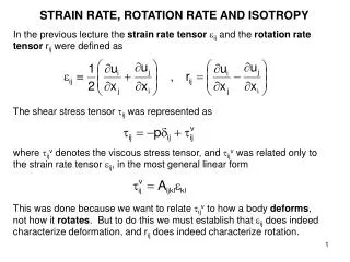
STRAIN RATE, ROTATION RATE AND ISOTROPY. In the previous lecture the strain rate tensor ij and the rotation rate tensor r ij were defined as. The shear stress tensor ij was represented as.

E N D
STRAIN RATE, ROTATION RATE AND ISOTROPY In the previous lecture the strain rate tensor ij and the rotation rate tensor rij were defined as The shear stress tensor ij was represented as where ijv denotes the viscous stress tensor, and ijv was related only to the strain rate tensor ij, in the most general linear form This was done because we want to relate ijv to how a body deforms, not how it rotates. But to do this we must establish that ij does indeed characterize deformation, and rij does indeed characterize rotation.
STRAIN RATE, ROTATION RATE AND ISOTROPY A deformable body may be deformed in two ways: extension shearing. Extensional deformation is illustrated below: Shear deformation is illustrated below:
STRAIN RATE, ROTATION RATE AND ISOTROPY We first consider extensional deformation. A moving deformable body has length x1 in the x1 direction. The velocity u1 is assumed to be changing in the x1 direction, so that the values on the left-hand side and right-hand side of the body are, respectively is In time t the left boundary moves a distance u1t, and the right boundary moves a distance [u1 + (u1/x1)x1]t
STRAIN RATE, ROTATION RATE AND ISOTROPY The initial length of the body is x1. The length of the body after time t is given as The extensional strain rate is the rate of length increase of the body per unit initial length per unit time = [(new length) – (old length)]/(old length)/(t) =
STRAIN RATE, ROTATION RATE AND ISOTROPY Note that u1/x1 > 0 for an elongating body and u1/x1 < 0 for a shortening body. The corresponding extensional strain rates in the x2 and x3 directions are, respectively, These extensional strain rates relate to the diagonal components of the strain rate tensor 11, 22 and 33 as follows:
STRAIN RATE, ROTATION RATE AND ISOTROPY Now we consider shear deformation. Consider the points A, B and C below. The velocities in the x1 direction at points A and C are, respectively, and the velocities in the x2 direction at points A and B are, respectively, C A B
STRAIN RATE, ROTATION RATE AND ISOTROPY • The body undergoes shear deformation over time t. That is: • Point A moves a distance u1t in the x1 direction and u2t in the x2 direction; • Point B moves a distance [u2 + (u2/x1)x1]t in the x2 direction; and • Point C moves a distance [u1 + (u1/x2)x2]t in the x1 direction.
STRAIN RATE, ROTATION RATE AND ISOTROPY Recall that for small angle , sin . The angles and created in time t are defined below. These can be approximated as:
STRAIN RATE, ROTATION RATE AND ISOTROPY The strain rate due to shearing can be defined as the angle increase rate ( + )/t, or thus
STRAIN RATE, ROTATION RATE AND ISOTROPY The strain rate due to shearing due to shearing d( + )/dt in the x1-x2 plane is related to the component 12 of the strain rate tensor as The corresponding components of the strain rate tensor due to shearing in the x2-x3 and x1-x3 planes are correspondingly
C STRAIN RATE, ROTATION RATE AND ISOTROPY It is thus seen that the strain rate tensor ij does indeed characterize the rate at which a body is deformed by elongation or shearing. We now must establish that the tensor does indeed characterize rotation. We approach this indirectly, by first defining circulation. Circulation is an integral measure of the tendency of a fluid to rotate. Let C denote some fixed closed circuit within a fluid (across which fluid can flow freely), and let denote an elemental arc length tangential to the circuit that is positive in the counterclockwise direction. The circulation is defined as:
1 2 3 4 STRAIN RATE, ROTATION RATE AND ISOTROPY To illustrate the idea of circulation, we consider two simple examples. The first of these is constant, rectilinear flow in the x direction with velocity U, so that (u, v, w) = (U, 0, 0). The circuit has length L in the x direction and length H in the y direction. The circulation around the circuit is: H U Thus the is no circulation around a circuit in rectilinear flow. L
1 2 3 4 STRAIN RATE, ROTATION RATE AND ISOTROPY Now we consider the case of plane Couette flow with Note that u = 0 where y = 0 and u = U where y = H. Now H U Thus there is circulation, and it is negative (i.e. directed in the clockwise direction). L
STRAIN RATE, ROTATION RATE AND ISOTROPY The concept of circulation is closely related to the concept of vorticity. Consider a loop around a region with area dA, such that the circulation around the circuit is d. The vorticity is defined as The vorticity of a fluid at a point is equal to twice the angular velocity of the fluid particles at that point. This can be seen by considering a fluid particle rotating with angular speed , at the center of a circle with radius dr. The arc length of the periphery of the circle is 2dr, the area of the circle is (dr)2, and the peripheral velocity is dr. Thus dr
1 2 3 4 STRAIN RATE, ROTATION RATE AND ISOTROPY The vorticity can be related to the velocity field as follows. Consider the elemental rectangular circuit below. The components of velocity at the center of the rectangle are (u, v). The component of the velocity normal to the circuit on segments 1, 2, 3 and 4 are 1. 2. 3. 4. y (u,v) Thus x
1 2 3 4 STRAIN RATE, ROTATION RATE AND ISOTROPY Reducing, And thus since = d/dA, y (u,v) x
STRAIN RATE, ROTATION RATE AND ISOTROPY Now we return to constant rectilinear flow and plane Couette flow. For rectilinear flow (u, v, w) = (U, 0, 0) and Therefore the illustrated red paddle will not rotate as it moves with the flow. For plane Couette flow (u, v, w) = (Uy/H, 0, 0) and The illustrate red paddle will thus rotate in the clockwise direction as it moves with the flow, with angular speed = U/(2H).
STRAIN RATE, ROTATION RATE AND ISOTROPY So far we have considered only 2D flows in the (x, y) plane, in which case angular velocity and vorticity are directed along the z axis. The appropriate 3D extension is Or expanding out Thus for example
STRAIN RATE, ROTATION RATE AND ISOTROPY The rate of rotation tensor rij is directly related to the vorticity vector i and thus to the angular velocity i. That is, (Note: do not confuse the Levi-Civita third-order tensor ijk with the strain rate tensor ij.)
STRAIN RATE, ROTATION RATE AND ISOTROPY Our goal is to relate the viscous stress tensor ijv to a measure of the rate of deformation not the rate of rotation, of a fluid. Thus we relate ijv to ij rather than ui/xj. The most general linear relation between ijv and ij is • The relation can be simplified by assuming that it is • isotropic, so that the form of the relation is invariant to coordinate rotation, and has the same physics in any direction, and • symmetric, so that ijv = jiv. We do not go through the complete details of isotropy here. We showed in Lecture 2, however, that pressure p is isotropic. More specifically, where ijp denotes the part of the stress tensor associated with pressure,
STRAIN RATE, ROTATION RATE AND ISOTROPY The most general second-order isotropic tensor Aij takes the form where C is an arbitrary scalar. (In the case of ijp, C = -p.) It turns out that the most general fourth-order isotropic tensor is (Aris, 1962) where again C1, C2 and C3 are arbitrary scalars. Thus the relation reduces to But for an incompressible fluid
STRAIN RATE, ROTATION RATE AND ISOTROPY Thus But But ij is a symmetric tensor, i.e. ij = ji. Further defining C2+ C3 = 2, where = the dynamic viscosity of the fluid, the relation reduces to or The above relation defines the constitutive relation for a viscous Newtonian fluid. Note that the form guarantees symmetry in ij.
STRAIN RATE, ROTATION RATE AND ISOTROPY Reference Aris, R. (1962) Vectors, Tensors and the Basic Equations of Fluid Mechanics. Prentice-Hall.