Download
1 / 16
170 likes | 202 Views
Understand cointegration in econometrics through formal and informal methods, such as CRDW and CRDF tests, to identify long-run relationships between variables. Learn how to test for cointegration using statistical tools like regression analysis and Durbin-Watson statistic. Explore the advantages and disadvantages of these tests.

E N D
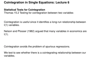
Cointegration in Single Equations: Lecture 6 • Statistical Tests for Cointegration • Thomas 15.2 Testing for cointegration between two variables • Cointegration is useful since it identifies a long-run relationship between I(1) variables. • Nelson and Plosser (1982) argued that many variables in economics are I(1). • Cointegration avoids the problem of spurious regressions. • We test to see whether there is a cointegrating relationship between our variables.
Cointegration in Single Equations • Main Task • First establish that two series are I(1) i.e. difference stationary. • If both Ytand Xt are I(1), there exists the possibility of a cointegrating relationship. • If two variables are integrated of different orders, say one is I(2) and other is I(1), there will not be cointegration. • Assuming both Ytand Xt are I(1), we estimate regression of Yt on a constant andXt • Yt = β0 + β1Xt + ut (1)
Cointegration in Single Equations • Main Task • We have both formal and informal methods of establishing cointegration based on the regression residuals ut from equation • Yt = β0 + β1Xt + ut (1) • (a) Informal:Plot the time series of the regression residuals ut and correlogram (i.e. autocorrelation function). • Are they stationary? • (b) Formal: Test directly if the disequilibrium errors are I(0). • ut=Yt - β0 - β1Xt • If utis I(0) then an equilibrium relationship exists. • And hence we have evidence of cointegration.
Testing for Cointegration • (1) Cointegrating Regression Durbin Watson (CRDW) Test • Suggested by Engle and Granger (1987). • Makes use of Durbin-Watson statistic • – similar to Sargan and Bhargava (1983) test for stationarity. • Test residuals from regression Yt = β0 + β1Xt + ut using DW stat. • Low Durbin-Watson statistic indicates no cointegration. • Similar to spurious regression result where the Durbin-Watson statistic was low for non-sense regression.
Testing for Cointegration • (1) Cointegrating Regression Durbin Watson (CRDW) Test • At 0.05 per cent significance level with sample size of 100, • the critical value is equal to 0.38. • Ho: DW = 0 => no cointegration (i.e. DW stat. is less than 0.38) • Ha: DW > 0 => cointegration (i.e. DW stat. is greater than 0.38) • Ho:ut = ut-1 + zt-1 • Ha:ut = ρut-1 + zt-1 ρ < 1 • N.B. Assumes that the disequilibrium errors ut can be modelled by a first order AR process. • Is this a valid assumption? • May require a more complicated model.
Testing for Cointegration • (2) Cointegrating Regression Dickey Fuller (CRDF) Test • Again based on OLS estimates of static regression • Yt = β0 + β1Xt + ut • We then test regression residuals ut under the null of nonstationarity against the alternative of stationarity using Dickey Fuller type tests. • Stationary residuals imply cointegration.
Testing for Cointegration • (2) Cointegrating Regression Dickey Fuller (CRDF) Test • Use lagged differenced terms to avoid serial correlation. • Δut = φ* ut-1 + θ1Δut-1 + θ2Δut-2 + θ3Δut-3 + θ4Δut-4 + et • Use F-test of model reduction and also minimize Schwarz Information Criteria. • Critical Values (CV) are from MacKinnon (1991) • Ho: φ* = 0 => no cointegration (i.e. TS is greater than CV) • Ha: φ* < 0 => cointegration (i.e. TS is less than CV)
Testing for Cointegration • Advantages of (CRDF) Test • Engle and Granger (1987) compared alternative methods for testing for cointegration. • (1) Critical values depend on the model used to simulated the data. • CRDF was least model sensitive. • (2) Also CRDF has greater power (i.e. most likely to reject a false null) compared to the CRDW test.
Testing for Cointegration • Disadvantage of (CRDF) Test • - Although the test performs well relative to CRDW test • there is still evidence that CRDF have absolutely low power. • Hence we should show caution in interpreting the results.
Testing for Cointegration • Example: Are Y and X cointegrated? • First be satisfied that the two time series are I(1). • E.g. apply unit root tests to X and Y in turn.
Testing for Cointegration • Once we are satisfied X and Y are both I(1), and hence there is the possibility of a cointegrating relationship, we estimate our static regression model. • Yt = β0 + β1Xt + ut • EQ( 1) Modelling Y by OLS (using Lecture 6a.in7) • The estimation sample is: 1 to 99 • Coefficient Std.Error t-value t-prob Part.R^2 • Constant 4.85755 0.1375 35.3 0.000 0.9279 • X 1.00792 0.005081 198. 0.000 0.9975 • sigma 0.564679 RSS 30.9296673 • R^2 0.997541 F(1,97) = 3.935e+004 [0.000]** • log-likelihood -82.8864 DW 2.28 • no. of observations 99 no. of parameters 2 • CRDW test statistic = 2.28 >> 0.38 = 5% critical value. • This suggests cointegration - assumes residuals follow AR(1) model.
Testing for Cointegration • After estimating the model save residuals from static regression. • (In PcGive after running regression click on Test and Store Residuals) • Informally consider whether stationary.
Testing for Cointegration • Using CRDF we incorporate lagged dependent variables into our regression • Δut = φ* ut-1 + θ1Δut-1 + θ2Δut-2 + θ3Δut-3 + θ4Δut-4 + et • And then assess which lags should be incorporated using model reduction tests and Information Criteria. • Progress to date • Model T p log-likelihood SC HQ AIC • EQ( 2) 94 5 OLS -74.238306 1.8212 1.7406 1.6859 • EQ( 3) 94 4 OLS -74.793519 1.7847 1.7202 1.6765 • EQ( 4) 94 3 OLS -74.797849 1.7364 1.6881 1.6553 • EQ( 5) 94 2 OLS -74.948145 1.6913 1.6591 1.6372 • EQ( 6) 94 1 OLS -75.845305 1.6621 1.6459 1.6350 • Tests of model reduction (please ensure models are nested for test validity) • EQ( 2) --> EQ( 6): F(4,89) = 0.77392 [0.5450] • EQ( 3) --> EQ( 6): F(3,90) = 0.67892 [0.5672] • EQ( 4) --> EQ( 6): F(2,91) = 1.0254 [0.3628] • EQ( 5) --> EQ( 6): F(1,92) = 1.7730 [0.1863] • Consequently we choose Δut = φ* ut-1 + et All model reduction tests are accepted hence move to most simple model
Testing for Cointegration • The estimated results from our model Δut = φ* ut-1 + et are as follows • EQ( 6) Modelling dresiduals by OLS (using Lecture 6a.in7) • The estimation sample is: 6 to 99 • Coefficient Std.Error t-value t-prob Part.R^2 • residuals_1 -1.16140 0.1024 -11.3 0.000 0.5805 • sigma 0.545133 RSS 27.6367834 • log-likelihood -75.8453 DW 1.95 • Which meansΔut = -1.161ut-1 + et • (-11.3) • CRDF test statistic = -11.3 << -3.39 = 5% Critical Value from MacKinnon. • Hence we reject null of no cointegration between X and Y.
Testing for Cointegration: Summary • To test whether two I(1) series are cointegrated we examine whether the residuals are I(0). • (a) We firstly use informal methods to see if they are stationary • (1) plot time series of residuals • (2) plot correlogram of residuals • (b) Two formal means of testing for cointegration. • (1) CRDW - Cointegrating Regression Durbin Watson Test • (2) CRDF - Cointegrating Regression Dickey Fuller Test
Next Lecture: Preview • In the next lecture we consider • - the relationship between cointegration and error correction models. • - we illustrate how the disequilibrium errors from a cointegrated regression can be incorporated in a short run dynamic model. • - What happens when we have more than two variables. • Do you have one cointegrating relationship between say three variables? Do we have more than one cointegrating relationship?