Biological variation
Biological variation. Biological variation. Biological variation Introduction Estimation (ANOVA application) Index-of-individuality Comparison of a result with a reference interval ("Grey-zone") Reference change value (RCV). Biological variation. Biological variation.


Biological variation
E N D
Presentation Transcript
Biological variation Biological variation • Biological variation • Introduction • Estimation (ANOVA application) • Index-of-individuality • Comparison of a result with a reference interval ("Grey-zone") • Reference change value (RCV) Statistics & graphics for the laboratory
Biological variation Biological variation • Reference interval and biological variation • Reference interval encompasses: • pre-analytical imprecision • analytical imprecision • within-subject biological variation • between-subject biological variation • Usefulness of reference intervals • Reference intervals are of most use • when the between-subject variation is smaller than the within-subject variation: • CVB-S < CVW-S, or CVW-S/CVB-S >1 • If not, individuals may have values which lie within reference limits but are highly unusual for them: See also later: Index of individuality • Uses of biological variation • Setting desirable analytical goals • Assessing significance of changes in serial results • Assessing utility of population based reference values • Deciding number of specimens required to assess homeostatic set point of an individual • Determining optimum mode for result reporting • Comparing available tests • Assessing clinical utility of tests • Abbreviations for biological variation • CVW-S = Within-subject • CVB-S = Between-subject • CVG = "Group" = SQRT(CV2W-S + CV2B-S) = ¼ of the reference interval • Note: sometimes CVG is used to designate CVB-S (e.g. in the Westgard database on analytical specifications) Statistics & graphics for the laboratory
Biological variation Estimation of biological variation (ANOVA-application) • Approaches • One overall analysis using nested ANOVA based ondedicated software (SAS, SPSS, BMDP etc.). • Stepwise approach with computation of variances at each level. • General requirement: Repeated measurements at each level, i.e. at least duplicates, in order to resolve the variance components. • a time period. • Inspection of data on biological variation • Generally, ANOVA is robust towards moderate deviations from normality, but it is sensitive towards outliers. • Occurrence of outliers • Within subgroups or one subgroup versus the bulk of the rest of subgroups • Within-subject variation • Homogeneity/heterogeneity • Within- & between subject biological variation • Example Creatinine Statistics & graphics for the laboratory
Biological variation Analytical & biological variation • Estimation of biological variation • Remark • Consider the importance of analytical imprecision. • Inter (B-S)/intra (W-S)-individual biological variation • Analytical variation (A) • Total dispersion of a single measurement of individuals*: • T2 = B-S2+ (W-S2+ A2) = B-S2 + T, W-S2 • Index of individuality (Ii)(see also later): • T,W-S/B-S~ W-S/B-S • *Ignoring pre-analytical variation • Components of variation-ANOVA • Between (B-S)- and within-individual(W-S) biological variation* • Inclusive analytical variation (σT,W-S) • The within-biological variation is here obtained as an average value for all the studied individuals, which generally is preferable. Statistics & graphics for the laboratory
Biological variation Analytical & within biological variation • Analytical variation can be minimized by collecting and running the samples within one run. • Shortcut computational principles • Duplicate sets of measurements • SD = [Σd2/2n]0.5 • for n duplicate measurements, • where dis the difference between pairs of measurements. • Examples • Measurements of duplicate samples to derive the SDA • Duplicate samples from each individual to derive SDT,W-S • Practical approach • Obtain repeated samples over a suitable time period, e.g. 5 samples, from a collection of individuals, e.g. 10-20 subjects, and measure each sample in duplicate. • Inspect/test data for outliers and variance homogeneity. • Carry out a simple ANOVA on the means of duplicates and derive SDB-S and SDT,W-S • Derive SDA from duplicates • Derive SDW-S from the relation: • SDT,W-S2 = 0.5 SDA2+ SDW-S2 • (the factor 0.5 enters because the means of duplicate measurements entered the analysis) Cochran&Bartlett; ANOVA Statistics & graphics for the laboratory
Biological variation Index-of-individuality (II) • Index-of-individuality (II) • CVW-S/CVB-S • is called • "Index-of-individuality" = • Ratio between within- and between-subject variation • Often, the analytical variation is included, to give • II = (CVW-S2 + CVA2)½/CVB-S • Harris EK Clin Chem 1974;20:1535-42 • Examples • Calculation of CVG • Range = 27 • Mean = 18 • ¼ of the RI in % of the mean = 36% Statistics & graphics for the laboratory
Biological variation Index-of-individuality (II) • II = CVW-S/CVB-S • If II < 0.6 • high degree of individuality • reference ranges of limited utility (better use RCV!) • If II > 1.4 • low degree of individuality • reference ranges are more useful • Most analytes have II < 1.4 !! • Examples Statistics & graphics for the laboratory
Biological variation Comparison of a result with a reference-interval • The "grey-zone" • Example • 2 measurement results for serum glucose: • (1) 88 mg/100 ml • (2) 109 mg/100 ml • with a reference-interval: 60 - 100 mg/100 ml. • Question: Is result (1) actually inside, result (2) outside the reference-interval? • Data : CVa = 2 %; CVi = 6.1 % • CVtot = SQRT(CVa2 +CVi2) = SQRT(2 • 2 + 6.1 • 6.1) = 6.4% • Transform CVtot into stot: 6.4 mg/100 ml (at 100 mg/100 ml) • Calculate the “grey-zone” around the limit of 100 mg/100 ml with 95 (90) % probability (Note: one-sided): • ±1.65 (1.29) stot or 1.65 (1.29) 6.4 mg/100 ml = ±10.6 (8.3) mg/100 ml. • Grey zone at 95 % = 89.4 - 110.6 mg/100 ml • Grey zone at 90 % = 91.7 - 108.3 mg/100 ml. • Thus, result (1) lies inside the reference-interval in both cases. • Result (2) lies outside the reference-interval only in the case of 90% probability. • Conclusion: • If one wants to miss few pathological cases, one would calculate the grey zone below the limit with 95 % probability, the one above the limit with 90 %. • Glucose – "Grey-zone" • Alternative approach • With the statistical concept of Power: How big is the chance that we decide "healthy", when the patient is sick, in fact (ß-error; false negatives). • The power concept will be explained later. It is important for: • Sample size method comparison • Limit of detection (LOD) • IQC Statistics & graphics for the laboratory
Biological variation "Grey zone" for results at reference limits P = 95% Biology, only 1.65 • CVW-S P = 95% Total 1.65 • [UA2+CVW-S2] UA Analytical uncertainty (see "Goals") Statistics & graphics for the laboratory
Biological variation • Reference Change Value (RCV), or Medically significant difference (Dmed) • 95 % interval for difference between two samplings and measurements Dmed = 1.96•[2•(CV2W-S+CV2Anal)]½ • The RCV is particular important for analytes with high CVB-S. • med for the “creatinine clearance” • C : ml plasma cleared per min per standard body surface • Ucr : concentration of creatinine in urine (mg/ml) • Pcr : concentration of creatinine in plasma (mg/ml) • V : volume urine flow in ml per min • A : body surface in m2 • For • Ucr : 1 mg/ml • Pcr : 0.01mg/ml • V : 1 ml/min • A : 1.88 m2 (man of 70 kg and 1.75 m tall) • is C = 92 ml/min/1.73 m2 • Calculation of sa: • When CVa = 2% for Ucr=1 mg/ml, then sa = 0.02 mg/ml. • When CVa = 2% for Pcr= 0.01 mg/ml, then sa = 0.0002 mg/ml. • CVa for V is not considered. • Note: in our example, sy = sa; y = C • sa = 92 • 0.0283 = 2.6 ml/min/1.73m2 Statistics & graphics for the laboratory
= 5.3 ml/min/1.73 m2 = 14.7 ml/min/1.73 m2 = 40.7 ml/min/1.73 m2 Biological variation med for the “creatinine clearance” • Calculation: • CVi = 15 % or at C = 92 ml/min/1.73 m2 , si = 13.8 ml/min/1.73 m2 (*) • stot = SQRT[2.62 + 13.82] = 14 ml/min/1.73m2 • Thus: Dmed = 1.96 • SQRT[2] • 14 = 38.9 ml/min/1.73 m2 • in other words a decrease in creatinine clearance of 42% is to consider medically significant. • (*) Tietz Textbook of Clinical Chemistry 2nd Ed, Burtis CA, Ashwood ER, eds. WB Saunders Company, Philadelphia, 1994: p 1536. • Note: If we also take the CVa for V into account, f.e. 5%, then : • This example thus makes it obvious that in particular the biological variation contributes to the medically signifcant value. It is for that reason that Tietz recommends: “...Sequential determinations of creatinine clearance and averaging of values are required to reduce this variation appreciably”. Statistics & graphics for the laboratory
Notes Notes Statistics & graphics for the laboratory