Download
1 / 21
210 likes | 418 Views
Adaptive Problem-Solving for Large-Scale Scheduling Problems: A Case Study by Jonathan Gratch and Steve Chien Published in JAIR, 1996. EARG presentation Oct 3, 200 8 by Frank Hutter. Overview. Problem domain Cool: scheduling for the deep space network Scheduling algorithm

E N D
Adaptive Problem-Solving for Large-Scale Scheduling Problems: A Case StudybyJonathan Gratch and Steve ChienPublished in JAIR, 1996 EARG presentation Oct 3, 2008by Frank Hutter
Overview • Problem domain • Cool: scheduling for the deep space network • Scheduling algorithm • Branch & Bound with a Lagrangian relaxation at each search node • Adaptive Problem Solving • Automatic Parameter Tuning by Local Search • Already contains many good ideas, 12 years ago!
Domain: Scheduling for the Deep Space Network • Collection of ground-based radio antennas • Maintain communication with research satellites and deep space probes • NASA’s Jet Propulsion Laboratory (JPL): automate scheduling of 26-meter subnet • Three 26-meter antennas • Goldstone, CA, USA • Canberra, Australia • Madrid, Spain
Scheduling problem“When should which antenna talk to which satellite?” • Project requirements • Number of communication events per period • Duration of communication events • Allowable gap between communication events • E.g. Nimbus-7 (meteorogical satellite): needs at least four 15-minute slots per day, not more than 5 hours apart • Antenna constraints • Only one communication at once • Antenna can only communicate with satellites in view • Routine maintenance antenna offline
Problem formulation • 0-1 integer linear programming formulation • Time periods: 0-1 integer variables (in/out) • Typical problem: 700 variables, 1300 constraints • Scheduling has to be fast • So human user can try “what if” scenarios • “For these reasons, the focus of development is upon heuristic techniques that do not necessarily uncover the optimal schedule, but rather produce adequate schedules quickly.” • Alas, they still don’t use local search ;-)
Scheduling algorithm • Branch and Bound (“Split-and-prune”) • At each node: • arc consistency (check all constraints containing time period just committed) • Lagrangian relaxation: each antenna by itself • Can be solved in linear time (dynamic programming for each antenna to get “non-exclusive sequence of time periods with maximum cumulative weight”)
Lagrangian relaxation • Relax project constraints, penalize violation by weight uj ; weight search for best vector u
Search Algorithm Parameters • Constraint ordering: • “Choose a constraint that maximally constrains the rest of the search space” • 9 heuristics, same 9 as secondary tie-breakers • Value ordering: “maximize the number of options available for future assignments” • 5 heuristics implemented • Weight search (for weight vector u) • 4 methods implemented • Refinement methods • 2 options: Standard B&B vs. (A=x fails, then try B=y instead of A=1-x --- does this have a name??)
Problem distribution • Not many problem instances available • Syntactic manipulation of set of real problems • Yields 6,600 problem instances • Only use subset of these 6,600 instances • Some generated instances seemed much harder than original instances • Discard “intractable” instances (original or generated) • Intractable: instances taking longer than 5 minutes
Determination of Resource Bound • Only 12% of problems unsolved in 5 minutes were solved in an hour • Reference to statistical analysis for that factor • should read that in EARG (Etzioni & Etzioni, 1994)
Adaptive Problem Solving: Approaches • Syntactic approach • Transform into more efficient form, using only syntactic structure • Recognize structural properties that influence effectiveness of different heuristic methods • Big lookup table, specifying heuristic to use • Somewhat similar to SATzilla Lin should look into it • (I think: includes newer research on symmetry breaking, etc) • Generative approach • Generate new heuristics based on partial runs of solver focus on inefficiencies in previous runs • “Often learning is within an instance and does not generalize to distributions of problems” • Statistical approach • Explicitly reason about performance of different heuristics across distribution of problems • Often: statistical generate-and-test approaches • Widely applicable (domains, utility functions) • Computationally expensive; local optima ( ParamILS)
Adaptive Problem Solving: Composer • Statistical approach • Generate-and-test hillclimbing • When evaluating a move: • Perform runs with neighbour • Collect differences in performance • Perform test to see if mean(differences) < 0 or >0 • Test assumes Normal distribution of differences • Terminate in first local optimum • Evaluation: • On large set of test instances (1000)
Meta-Control Knowledge in Composer: Layered Search • Order parameters by their importance • First only allow move in the first level, then allow move in the second level, etc • Not sure whether they iterate • Levels • Level 0: weight search method • Level 1: Refinement method • Level 2: Secondary refinement, value ordering • Level 3: Primary constraint ordering • (this comes last since they strongly believed their manual one was best – it was indeed chosen)
Empirical evaluation • Setting of Composer parameters • = 0.05, n0 = 15 (empirically determined) • Training set: 300 problem instances • Test set: 1000 problem instances • They say “independent”, but I don’t think disjoint • Stochasticity from drawing instances at random • Estimate expected performance as average over multiple experimental trials • But don’t tell us how many trials they did • Measure performance every 20 samples
My view of their approach • Some very good ideas, already 12 years ago • Proper use of training/test set • Statistical test for move is interesting • Problems I see • If a move neither decreases nor increases expected utility, the statistical test can force “an infinite number” of evaluations • Even if this just decides between two poor configurations • Stuck in local minima • Never re-using instances? Once they’re out of instances, they stop (also still a little unclear)