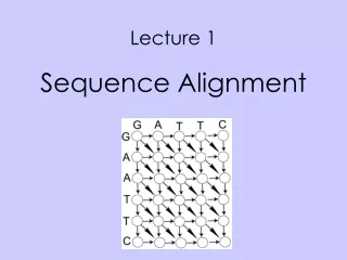
Sequence Alignment I Lecture #2

1. Sequence Alignment ILecture #2 Background Readings: Gusfield, chapter 11. Durbin et. al., chapter 2. This class has been edited from Nir Friedman’s lecture which is available at www.cs.huji.ac.il/~nir. Changes made by Dan Geiger, then Shlomo Moran, and finally Benny Chor. .

2. Sequence Comparison Much of bioinformatics involves sequences • DNA sequences • RNA sequences • Protein sequences We can think of these sequences as strings of letters • DNA & RNA: alphabet ∑of 4 letters (A,C,T/U,G) • Protein: alphabet ∑ of 20 letters (A,R,N,D,C,Q,…)

3. g1 g2 Sequence Comparison (cont) • Finding similarity between sequences is important for many biological questions For example: • Find similar proteins • Allows to predict function & structure • Locate similar subsequences in DNA • Allows to identify (e.g) regulatory elements • Locate DNA sequences that might overlap • Helps in sequence assembly

4. Sequence Alignment Input:two sequences over the same alphabet Output: an alignment of the two sequences Example: • GCGCATGGATTGAGCGA • TGCGCCATTGATGACCA A possible alignment: -GCGC-ATGGATTGAGCGA TGCGCCATTGAT-GACC-A

5. Alignments -GCGC-ATGGATTGAGCGA TGCGCCATTGAT-GACC-A Three “components”: • Perfect matches • Mismatches • Insertions & deletions (indel) Formal definition of alignment:

6. Choosing Alignments There are many (how many?) possible alignments For example, compare: -GCGC-ATGGATTGAGCGA TGCGCCATTGAT-GACC-A to ------GCGCATGGATTGAGCGA TGCGCC----ATTGATGACCA-- Which one is better?

7. Scoring Alignments Motivation: • Similar (“homologous”) sequences evolved from a common ancestor • In the course of evolution, the sequences changed from the ancestral sequence by random mutations: • Replacements: one letter changed to another • Deletion: deletion of a letter • Insertion: insertion of a letter • Scoring of sequence similarity should reflect how many and which operations took place

8. A Naive Scoring Rule Each position scored independently, using: • Match: +1 • Mismatch : -1 • Indel -2 Score of an alignment is sum of position scores

9. Example -GCGC-ATGGATTGAGCGA TGCGCCATTGAT-GACC-A Score: (+1x13) + (-1x2) + (-2x4) = 3 ------GCGCATGGATTGAGCGA TGCGCC----ATTGATGACCA-- Score: (+1x5) + (-1x6) + (-2x11) = -23 according to this scoring, first alignment is better

10. More General Scores • The choice of +1,-1, and -2 scores is quite arbitrary • Depending on the context, some changes are moreplausible than others • Exchange of an amino-acid by one with similar properties (size, charge, etc.) vs. • Exchange of an amino-acid by one with very different properties • Probabilistic interpretation: (e.g.) How likely is one alignment versus another ?

11. Additive Scoring Rules • We define a scoring function by specifying • (x,y) is the score of replacingx by y • (x,-) is the score of deletingx • (-,x) is the score of insertingx • The score of an alignment is defined as the sum of position scores

12. The Optimal Score • The optimal (maximal) score between two sequences is the maximal score of all alignments of these sequences, namely, • Computing the maximal score or actually finding an alignment that yields the maximal score are closely related tasks with similar algorithms. • We now address these problems.

13. Computing Optimal Score • How can we compute the optimal score ? • If |s| = n and |t| = m, the number A(m,n) of possible alignments is large! Exercise: Show that • So it is not a good idea to go over all alignments • The additive form of the score allows us to apply dynamic programming to compute optimal score efficiently.

14. Recursive Argument • Suppose we have two sequences:s[1..n+1] and t[1..m+1] The best alignment must be one of three cases: 1. Last match is (s[n+1],t[m +1] ) 2. Last match is (s[n +1],-) 3. Last match is (-, t[m +1] )

15. Recursive Argument • Suppose we have two sequences:s[1..n+1] and t[1..m+1] The best alignment must be one of three cases: 1. Last match is (s[n+1],t[m +1] ) 2. Last match is (s[n +1],-) 3. Last match is (-, t[m +1] )

16. Recursive Argument • Suppose we have two sequences:s[1..n+1] and t[1..m+1] The best alignment must be one of three cases: 1. Last match is (s[n+1],t[m +1] ) 2. Last match is (s[n +1],-) 3. Last match is (-, t[m +1] )

17. Useful Notation (ab)use of notation: V[i,j] = value of optimal alignment between i prefix of s and j prefix of t.

18. Recursive Argument (ab)use of notation: V[i,j] = value of optimal alignment between i prefix of s and j prefix of t. • Using our recursive argument, we get the following recurrence for V:

19. T S Recursive Argument • Of course, we also need to handle the base cases in the recursion (boundary of matrix): AA - - versus We fill the “interior of matrix” using our recurrence rule

20. T S Dynamic Programming Algorithm We continue to fill the matrix using the recurrence rule

21. T S +1 -2 -A A- -2 (A- versus -A) Dynamic Programming Algorithm versus

22. T S Dynamic Programming Algorithm (hey, what is the scoring functions(x,y) ? )

23. T S Conclusion: V(AAAC,AGC) = -1 Dynamic Programming Algorithm

24. T S Reconstructing the Best Alignment • To reconstruct the best alignment, we record which case(s) in the recursive rule maximized the score

25. T S AAAC AG-C Reconstructing the Best Alignment • We now trace back a path that corresponds to the best alignment

26. T S AAAC -AGC AAAC AG-C Reconstructing the Best Alignment • More than one alignment could have the best score (sometimes, even exponentially many) AAAC A-GC

27. T S Time Complexity Space: O(mn) Time: O(mn) • Filling the matrix O(mn) • Backtrace O(m+n)

28. Space Complexity • In real-life applications, n and m can be very large • The space requirements of O(mn) can be too demanding • If m = n = 1000, we need 1MB space • If m = n = 10000, we need 100MB space • We can afford to perform extra computation to save space • Looping over million operations takes less than seconds on modern workstations • Can we trade space with time?

29. A G C 1 2 3 0 0 0 -2 -4 -6 1 -2 1 -1 -3 A 2 -4 -1 0 -2 A 3 -6 -3 -2 -1 A 4 -8 -5 -4 -1 C Why Do We Need So Much Space? To compute just the valueV[n,m]=V(s[1..n],t[1..m]), we need only O(min(n,m)) space: • Compute V(i,j), column by column, storing only two columns in memory (or line by line if lines are shorter). Note however that • This “trick” fails if we want toreconstruct the optimal alignment. • Trace back information requires keeping all back pointers, O(mn) memory.

30. Local Alignment The alignment version we studies so far is called global alignment: We align the whole sequence s to the whole sequence t. Global alignment is appropriate when s,t arehighly similar(examples?), but makes little sense if they are highly dissimilar. For example, when s (“the query”) is very short,butt (“the database”)is very long.

31. Local Alignment When s and t are not necessarily similar, we may want to consider a different question: • Find similar subsequences of s and t • Formally, given s[1..n] and t[1..m] find i,j,k, and l such that V(s[i..j],t[k..l]) is maximal • This version is called local alignment.

32. Local Alignment • As before, we use dynamic programming • We now want to setV[i,j] to record the maximum value over all alignments of a suffix of s[1..i] and a suffixof t[1..j] • In other words, we look for a suffix of a prefix. • How should we change the recurrence rule? • Same as before but with an option to start afresh • The result is called the Smith-Waterman algorithm, after its inventors (1981).

33. Local Alignment New option: • We can start a new match instead of extending a previous alignment Alignment of empty suffixes

34. T S Local Alignment Example s =TAATA t =TACTAA

35. T S Local Alignment Example s =TAATA t =TACTAA

36. T S Local Alignment Example s =TAATA t =TACTAA