Download
1 / 42
420 likes | 609 Views
ALGORITHMIC TRADING Hidden Markov Models. Overview. Introduction Methodology Programming codes Conclusion. a) Introduction. Markov Chain Named after Andrey Markov, Russian mathematician. Mathematical system that undergoes transitions from one state to another state.

E N D
Overview • Introduction • Methodology • Programming codes • Conclusion
a) Introduction • Markov Chain • Named after Andrey Markov, Russian mathematician. • Mathematical system that undergoes transitions from one state to another state. • From a finite or countable number of possible states in a chainlike manner. • Next state depends ONLY on the current state and not the past.
a) Introduction Simple 2 States Markov Chain Models
a) Introduction • System is in a certain state at each step. • States are changing randomly between steps. • Steps can be time or others measurements. • Random process is simply to map states to steps.
a) Introduction 1 2 Markov Property – The state at next step or all future steps, given its current state depends only on the current state. Transition Probabilities – Probability of transiting to various states.
a) Introduction • The Drunkard’s Walk • Random walk on the number line • At each step, position change by +1 or -1 or 0. • Depends only on current position.
a) Introduction • Transition Probability Matrix • Simple matrix holding all the state changing probabilities. • Eg: : Imagine that the sequence of rainy and sunny days is such that each day’s weather depends only on the previous day’s, and the transition probabilities are given by the following table.
a) Introduction if today is rainy, the probability that tomorrow will be rainy is 0.9; if today is sunny, that probability is 0.6. The weather is then a two-state Markov chain, with t.p.m. Γ given by: Γ = 0.9 0.1 0.6 0.4
a) Introduction to HMM • Hidden Markov Model • it is a Markov chain but the states are hidden, not observable. • In a normal Markov chain, t.p.m are the only parameters. In HMM, although state is not directly visible BUT the output which is dependent on the state is visible! • Thus the sequence of output reveals something about the sequence of states.
a) Introduction to HMM Therefore, what is available to the observer is another stochastic process linked to the Markov chain. The underlying Markov chain a.k.a the regime or state, will be directly affecting the distribution of the observed process.
a) Introduction to HMM • The Urn Problem • A genie is in a room that is not visible to you. It is drawing balls labeled y1, y2, y3, ... from the urns X1, X2, X3, ... in that room and putting the balls on a conveyor belt, where you can observe the sequence of the balls but not the sequence of urns from which they were chosen.
a) Introduction to HMM • The genie has some procedure to choose urns; the choice of the urn for the n-th ball depends upon only a random number and the choice of the urn for the (n − 1)-th ball. • Because the choice of urn does not directly depend on the urns further previous choices, this is called a Markov process with hidden states。
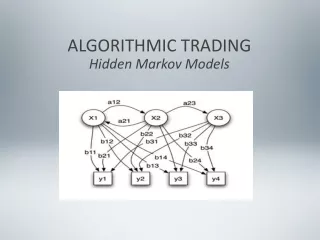
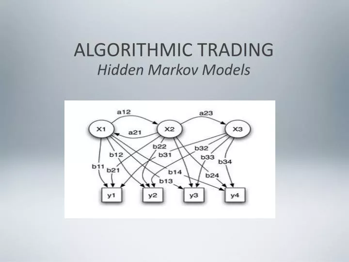
a) Introduction to HMM Probabilistic parameters of a hidden Markov model x — statesy — possible observationsa — state transition probabilitiesb — output probabilities
END OF INTRODUCTION! METHODOLOGY
Methodology Main Idea Total No. of data: 1400=1000+400
Markov Chain a22 = ? s2: Cloudy a12 = ? a23 = ? a21 = ? a32 = ? a13 = ? s1: Sunny s3: Rainy a31 = ? a11 = ? a33 = ?
Model—λ = {A,B,Π} A = {a11, a12, ..., aNN} : a transition probability matrix A, where each aij represents the probability of moving from state si to state sj B = bi(ot) : a sequence of observation likelihoods, also called emission probabilities, expressing the probability of an observation ot being generated from a state si at time t Π = {π1, π2, ..., πN} : an initial probability distribution, where πi indicates the probability of starting in state si.
Model—Other Parameters S = {s1, s2, ..., sN} a set of N hidden states, Q = {q1, q2, ..., qT } a state sequence of length T taking values from S, O = {o1, o2, ..., oT } an observation sequence consisting of T observations, taking values from the discrete alphabet V = {v1, v2, ..., vM},
Model—Likelihood:P(O|λ) Forward αt(i) = P(o1, o2, . . . , ot, qt = si|λ) Backward βt(i) = P(ot+1, ot+2, . . . , oT |qt = si, λ)
Model—Learning: Re-estimation ξt(i, j) = P(qt = si, qt+1 = sj |O, λ) γt(i) = P(qt = si|O, λ)
Applying HMM(Discrete) Model: Window length=100; N=3; M=; Initial parameter estimation: Random λ = {A,B,Π} Final model
Applying HMM(Discrete) Test Out of sample Generating trading signals Ot+1 & Ot : Trading strategy
Content A Ideas B Code Structure C Results D Limitations and TODOs
Section A - Ideas Parameter Estimation Prediction Trading Strategy
Parameter estimation-HMM A, B, pie 3 steps: likelihood, decoding, learning Greeks Updating, Iteration
the Choice of B Discrete - not smooth Time homogenous, why? a. Memory cost N * M * T (3 * 1000 * 100) in one iteration step b. Difficult to update Why continuous dist. can do this? a. Less parameters, less cost b. Update the time varying B directly
Parameter Updating How to compute updated B? Function get_index and its inverse function How to choose size of B? Extend the min and max, prepare to for extreme value. set a max, min, then interval length, set a function
Convergence Condition P converges to Po, set the eps Local maximum, not global
Prediction Find the q from last window -> the most likely state(t + 1) Find the B from last window -> the most likely obs given state Combine them to get most likely o(t + 1) Drawback: previous B to get new obs
Trading Strategy o(t + 1) > o(t) buy, otherwise sell set an indicator function I(buy or sell), which value is +1 when buy, -1 when sell Valuation: daily P&L = I * (true value(t + 1) - true value(t)) Sum daily P&L to get accumulate P&L, plot
section c - results P&L, window length = 30, state number = 3
Section b - Code Structure double update data {input = window length data output = a, b, pie in one step iteration, by using HMM} int main { generate a b pie( window length, state numbers) in uniformly distribution update data( 1~ window length) compute p, q update until p converges get best a, b, pie @ time 1 ~ window length use a, b, pie @ time period 1 as initialization, run update data iteration until p converges iteration until end of data prediction: q at last window b at last window to get most likely price @ time t + 1, say o(t + 1) our strategy backtesting and draw p & l (in Matlab for convenience) }
section c - results P&L, window length = 50, state number = 3
section c - results P&L, window length = 70, state number = 3
section c - results P&L, window length = 100, state number = 3
section d - drawbacks and todos Drawbacks: a. Iteration: Why we can use paras from last window to initialize paras of this window? b. Prediction: Why can use previous B to get next observation? c. Matrix B: time homogenous, does not make sense d. Discrete Distribution: Not smooth, not continuous... e. How many shares we will buy/sell?
todos a. Continuous Distribution and GMM b. More Trading Strategy: Computing expectation price rather than the most likely one because their are too many probabilities in a vector; their differences are slight -> more errors c. Transaction Cost: when o(t + 1) - o(t) >(<) c, buy/sell