Download

1 / 30
300 likes | 458 Views
Uncertainty in Sensing (and action). Planning With Probabilistic Uncertainty in Sensing. No motion. Perpendicular motion. The “Tiger” Example. Two states: s 0 (tiger-left) and s 1 (tiger right) Observations: GL (growl-left) and GR (growl-right) received only if listen action is chosen

E N D
Planning With Probabilistic Uncertainty in Sensing No motion Perpendicular motion
The “Tiger” Example • Two states: s0 (tiger-left) and s1 (tiger right) • Observations: GL (growl-left) and GR (growl-right) received only if listen action is chosen • P(GL|s0)=0.85, P(GR|s0)=0.15 • P(GL|s1)=0.15, P(GL|s1)=0.85 • Rewards: • -100 if wrong door opened, +10 if correct door opened, -1 for listening
Belief state • Probability of s0vs s1 being true underlying state • Initial belief state: P(s0)=P(s1)=0.5 • Upon listening, the belief state should change according to the Bayesian update (filtering) But how confident should you be on the tiger’s position before choosing a door?
Partially Observable MDPs • Consider the MDP model with states sS, actions aA • Reward R(s) • Transition model P(s’|s,a) • Discount factor g • With sensing uncertainty, initial belief state is a probability distributions over state: b(s) • b(si) 0 for all siS, i b(si) = 1 • Observations are generated according to a sensor model • Observation space oO • Sensor model P(o|s) • Resulting problem is a Partially Observable Markov Decision Process (POMDP)
Belief Space • Belief can be defined by a single number pt = P(s1|O1,…,Ot) • Optimal action does not depend on time step, just the value of pt • So a policy p(p) is a map from [0,1] {0,1,2} 0 1 listen open-left open-left open-right p
Utilities for non-terminal actions • Now consider p(p) listen for p [a,b] • Reward of -1 • If GR is observed at time t, p becomes • P(GRt|s1) P(s1 | p) / P(GRt|p) • 0.85 p / (0.85 p + 0.15 (1-p)) = 0.85p / (0.15 + 0.7 p) • Otherwise, p becomes • P(GLt|s1) P(s1 | p) / P(GLt| p) • 0.15 p / (0.15 p + 0.85 (1-p)) = 0.15p / (0.85 - 0.7 p) • So, the utility at p is • Up(p) = -1 + P(GR|p) Up(0.85p / (0.15 + 0.7 p)) + P(GL|p)Up(0.15p / (0.85 - 0.7 p))
POMDP Utility Function • A policy p(b)is defined as a map from belief states to actions • Expected discounted reward with policy p: Up(b) = E[t gtR(St)]where St is the random variable indicating the state at time t • P(S0=s) = b0(s) • P(S1=s) = ?
POMDP Utility Function • A policy p(b)is defined as a map from belief states to actions • Expected discounted reward with policy p: Up(b) = E[t gtR(St)]where St is the random variable indicating the state at time t • P(S0=s) = b0(s) • P(S1=s) = P(s|p(b0),b0) = s’ P(s|s’,p(b0)) P(S0=s’) = s’ P(s|s’,p(b0)) b0(s’)
POMDP Utility Function • A policy p(b)is defined as a map from belief states to actions • Expected discounted reward with policy p: Up(b) = E[t gtR(St)]where St is the random variable indicating the state at time t • P(S0=s) = b0(s) • P(S1=s) = s’ P(s|s’,p(b)) b0(s’) • P(S2=s) = ?
POMDP Utility Function • A policy p(b)is defined as a map from belief states to actions • Expected discounted reward with policy p: Up(b) = E[t gtR(St)]where St is the random variable indicating the state at time t • P(S0=s) = b0(s) • P(S1=s) = s’ P(s|s’,p(b)) b0(s’) • What belief states could the robot take on after 1 step?
b0 Choose action p(b0) b1 Predict b1(s)=s’ P(s|s’,(b0)) b0(s’)
b0 Choose action p(b0) b1 Predict b1(s)=s’ P(s|s’,(b0)) b0(s’) Receiveobservation oA oB oD oC
b0 Choose action p(b0) b1 Predict b1(s)=s’ P(s|s’,(b0)) b0(s’) Receiveobservation P(oA|b1) P(oB|b1) P(oC|b1) P(oD|b1) b1,A b1,B b1,C b1,D
b0 Choose action p(b0) b1 Predict b1(s)=s’ P(s|s’,(b0)) b0(s’) Receiveobservation P(oA|b1) P(oB|b1) P(oC|b1) P(oD|b1) b1,A b1,B b1,C b1,D Update belief b1,A(s) = P(s|b1,oA) b1,C(s) = P(s|b1,oC) b1,B(s) = P(s|b1,oB) b1,D(s) = P(s|b1,oD)
b0 Choose action p(b0) b1 Predict b1(s)=s’ P(s|s’,(b0)) b0(s’) P(o|b) = sP(o|s)b(s) Receiveobservation P(oA|b1) P(oB|b1) P(oC|b1) P(oD|b1) b1,A b1,B b1,C b1,D Update belief P(s|b,o) = P(o|s)P(s|b)/P(o|b) = 1/Z P(o|s) b(s) b1,A(s) = P(s|b1,oA) b1,C(s) = P(s|b1,oC) b1,B(s) = P(s|b1,oB) b1,D(s) = P(s|b1,oD)
Belief-space search tree • Each belief node has |A| action node successors • Each action node has |O| belief successors • Each (action,observation) pair (a,o) requires predict/update step similar to HMMs • Matrix/vector formulation: • b(s): a vector b of length |S| • P(s’|s,a): a set of |S|x|S| matrices Ta • P(ok|s): a vector ok of length |S| • ba= Tab(predict) • P(ok|ba) = okTba(probability of observation) • ba,k = diag(ok)ba / (okTba) (update) • Denote this operation as ba,o
Receding horizon search • Expand belief-space search tree to some depth h • Use an evaluation function on leaf beliefs to estimate utilities • For internal nodes, back up estimated utilities:U(b) = E[R(s)|b] + gmaxaA oO P(o|ba)U(ba,o)
QMDP Evaluation Function • One possible evaluation function is to compute the expectation of the underlying MDP value function over the leaf belief states • f(b) = sUMDP(s) b(s) • “Averaging over clairvoyance” • Assumes the problem becomes instantly fully observable after 1 action • Is optimistic: U(b) f(b) • Approaches POMDP value function as state and sensing uncertainty decreases • In extreme h=1 case, this is called the QMDP policy
Utilities for terminal actions • Consider a belief-space interval mapped to a terminating action p(p) open-right for p [a,b] • If true state is s1, reward is +10, otherwise -100 • P(s1)=p, so Up(p) = p*10 - (1-p)*100 Up 0 1 p open-right
Utilities for terminal actions • Now consider p(p) open-right for p [a,b] • If true state is s1, reward is -100, otherwise +10 • P(s1)=p, so Up(p) = -p*100 + (1-p)*10 Up 0 1 p open-left open-right
Piecewise Linear Value Function • Up(p) = -1 + P(GR|p) Up(0.85p / P(GR| p)) + P(GL|p) Up(0.15p / P(GL| p)) • If we assume Up at 0.85p / P(GR| p) and 0.15p / P(GL| p) are linear functions Up(x) = m1x+b1and Up(x) = m2x+b2, then • Up(p) = -1 + P(GR|p) (m1 0.85p / P(GR| p) + b1) + P(GL|p) (m2 0.15p / P(GL| p) + b2) = -1 + m10.85p + b1P(GR|p) + m20.15p + b2P(GL|p) = -1 + 0.15b1+0.85b2+ (m1 0.85 + m2 0.15 + 0.7 b1 - 0.7 b2) pLinear!
Value Iteration for POMDPs • Start with optimal zero-step rewards • Compute optimal one-step rewards given piecewise linear U Up 0 1 p open-left listen open-right
Value Iteration for POMDPs • Start with optimal zero-step rewards • Compute optimal one-step rewards given piecewise linear U Up 0 1 p open-left listen open-right
Value Iteration for POMDPs • Start with optimal zero-step rewards • Compute optimal one-step rewards given piecewise linear U • Repeat… Up 0 1 p open-left listen open-right
Worst-case Complexity • Infinite-horizon undiscounted POMDPs are undecideable (reduction to halting problem) • Exact solution to infinite-horizon discounted POMDPs are intractable even for low |S| • Finite horizon: O(|S|2 |A|h|O|h) • Receding horizon approximation: one-step regret is O(gh) • Approximate solution: becoming tractable for |S| in millions • a-vector point-based techniques • Monte Carlo tree search • …Beyond scope of course…
(Sometimes) Effective Heuristics • Assume most likely state • Works well if uncertainty is low, sensing is passive, and there are no “cliffs” • QMDP – average utilities of actions over current belief state • Works well if the agent doesn’t need to “go out of the way” to perform sensing actions • Most-likely-observation assumption • Information-gathering rewards / uncertainty penalties • Map building
Schedule • 11/27: Robotics • 11/29 Guest lecture: David Crandall, computer vision • 12/4: Review • 12/6: Final project presentations, review