Download
1 / 27
300 likes | 648 Views
Multiple Linear and Polynomial Regression with Statistical Analysis.

E N D
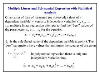
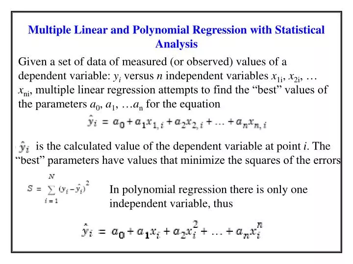
Multiple Linear and Polynomial Regression with Statistical Analysis Given a set of data of measured (or observed) values of a dependent variable: yi versus n independent variables x1i, x2i, … xni, multiple linear regression attempts to find the “best” values of the parameters a0, a1, …an for the equation is the calculated value of the dependent variable at point i. The “best” parameters have values that minimize the squares of the errors In polynomial regression there is only one independent variable, thus
Multiple Linear and Polynomial Regression with Statistical Analysis Typical examples of multiple linear and polynomial regressions include correlation of temperature dependent physical properties, correlation of heat transfer data using dimensionless groups, correlation of non-ideal phase equilibrium data and correlation of reaction rate data. The software packages enable high precision correlation of the data, however statistical analysis is essential to determine the quality of the fit (how well the regression model fits the data) and the stability of the model (the level of dependence of the model parameters on the particular set of data). The most important indicators for such studies are the residual plot (quality of the fit) and 95% confidence intervals (stability of the model)
Regression and Analysis of “Heat of Hardening” Data Woods et al(1932) investigated the integral heat of hardening of cement as a function of composition. The independent variables represent weight percent of the clinker compounds: x1-tricalcium aluminate (3CaO ·Al2O3),x2-tricalcium silicate (3CaO ·SiO2), x3-tetracalcium alumino-ferrite (4CaO ·Al2O3·Fe2O3), and x4- β-dicalcium silicate (3CaO ·SiO2). The dependent variable, y is the total heat evolved (in calories per gram cement) in a 180-day period.
Regression and Analysis of “Heat of Hardening” Data Calculate the coefficients of a linear model representation of y as function of x1, x2, x3, and x4, calculate the variance and the correlation coefficient R2 and the 95% confidence intervals. Prepare a residual plot. Consider the cases when the model includes and does not include a free parameter.
“Heat of Hardening” Data – Regression and Analysis by Polymath Non-zero intercept Model type
“Heat of Hardening” Data –Analysis of the Linear Model that Includes a Free Parameter Highly unstable model. All 95% confidence intervals larger in absolute value than the respective parameters. R2 value close to 1, indicates good fit between model and data. May be misleading occasionally. Rmsd and variance values used for comparison between different models
“Heat of Hardening” Data – Residual Plot of the Linear Model that Includes a Free Parameter Maximal error ~ 4% Random residual distribution indicates good fit between the model and the data
“Heat of Hardening” Data – Demonstration of the Harmful Effect of the Instability Last data point removed Removal of the last data point causes substantial change in all the parameter values. In case of the parameter a4 even its sign is changed
“Heat of Hardening” Data – A Stable Model is Obtained After Removing the Free Parameter Last data point removed
Correlation of Heat Capacity Data for Ethane A polynomial has to be fitted to heat capacity data provided by Ingham et al*. This data set includes 41 data points in the temperature range of 100 K – 400 K. The degree of the polynomial: where Cp is the heat capacity in J/kg-mol·K, T is the temperature in K, and a0, a1,... are the regression model parameters, which best represents the data, has to be found. The goodness of fit should be determined based on the variance, the correlation coefficient (R2), the confidence intervals of the parameters, and the residual plot. Ingham, H.; Friend, D.G.; Ely, J.F.; "Thermophysical Properties of Ethane"; J. Phys. Ref. Data 1991, 20, 275
Heat Capacity Data for Ethane, Fitting a 3rd Degree Polynomial Model type
Heat Capacity Data for Ethane, Fitting a 3rd Degree Polynomial All the parameters indicate satisfactory model. Note, however, the differences of orders of magnitude between the parameter values. This may limit the highest degree of polynomial to be fitted Rmsd and variance values used for comparison between different models
Heat Capacity Data for Ethane, Calculated (3rd Degree Polynomial)and Experimental Values On the scale of the entire range of the Cp data the fit seems to be excellent
Heat Capacity Data for Ethane, Residual Plot for the 3rd Degree Polynomial Maximal Error ~ 1% High resolution residual plot shows oscillatory behavior which is not explained by the 3rd degree polynomial
Heat Capacity Data for Ethane, Defining Standardized Temperature Values for High Order Polynomial Fitting
Heat Capacity Data for Ethane, Fitting a 5rd Degree Polynomial Using standardized values yields model parameters of similar magnitude, enables fitting higher order polynomials and improves considerably all the statistical indicators
Heat Capacity Data for Ethane, Residual Plot of a 5th Degree Polynomial Maximal Error ~ 0.03% Using standardized independent variable values enables fitting polynomials with precision higher than justified by the experimental error.
Modeling Vapor Pressure Data for Ethane A vapor pressure data set provided by Ingham et al* includes 107 data points in the temperature range of 92 K – 304 K. This temperature range covers almost completely the range between the tripe point temperature (= 90.352 K) and the critical temperature (TC = 305.32 K). The temperature dependence of the vapor pressure should be modeled by the Clapeyron, Antoine and Wagner equations The Clapeyron equation is a two parameter equation: where P is the vapor pressure (Pa), T –temperature (K) , A and B are parameters *Ingham, H.; Friend, D.G.; Ely, J.F.; "Thermophysical Properties of Ethane"; J. Phys. Ref. Data 1991, 20, 275
Modeling Vapor Pressure Data for Ethane by the Clapeyron Equation using Linear Regression = ln(P_Pa) = 1/T_K
Modeling Vapor Pressure Data for Ethane by the Clapeyron Equation using Linear Regression All the indicators show good, acceptable fit!
Modeling Vapor Pressure Data for Ethane by the Clapeyron Equation using Linear Regression Maximal error in ln(P) ~80% in P ~ 52% The residual plot reveals large unexplained curvature in the data
Modeling Vapor Pressure Data for Ethane by the Antoine Equation using Non-linear Regression Model type and solution algorithm Initial guess from Clapeyron eqn.
Modeling Vapor Pressure Data for Ethane by the Antoine Equation using Non-linear Regression Variance smaller by 2 orders of magnitude than Clapeyron Experimental and calculated values cannot be distinguished.
Modeling Vapor Pressure Data for Ethane by the Antoine Equation using Non-linear Regression Random residual distribution in the low pressure range, unexplained curvature in the high pressure range Maximal error in ln(P) ~1% in P ~ 5%
Modeling Vapor Pressure Data for Ethane with the Wagner Equation Where TR = T/TC is the reduced temperature PR = P/PC is the reduced pressure and τ = 1 - TR. For ethane TC = 305.32 K, PC =4.8720E+06 Pa In order to obtain the model parameters using linear regression the following variables are defined: Tr = T_K / 305.32 lnPr = ln(P_Pa / 4872000) t = (1 - Tr) / Tr t15 = (1 - Tr) ^ 1.5 / Tr t3 = (1 - Tr) ^ 3 / Tr t6 = (1 - Tr) ^ 6 / Tr
Modeling Vapor Pressure Data for Ethane with the Wagner Equation using Multiple Linear Regression Tr = T_K / 305.32 lnPr = ln(P_Pa / 4872000) t = (1 - Tr) / Tr t15 = (1 - Tr) ^ 1.5 / Tr t3 = (1 - Tr) ^ 3 / Tr t6 = (1 - Tr) ^ 6 / Tr
Modeling Vapor Pressure Data for Ethane with the Wagner Equation using Multiple Linear Regression Maximal Error in ln(Pr) ~ 0.6% Note random residuals distribution in the entire data range