Download
1 / 26
260 likes | 467 Views
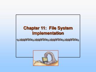
T 2m. t. The ELDAS system implementation and output production at Météo-France. Gianpaolo BALSAMO, François BOUYSSEL, Jöel NOILHAN. 2D-Var. ELDAS 2nd progress meetin g – INM Madrid 10-11 december 2003. Plan of the presentation. ELDAS at Météo-France The implementation of the system

E N D
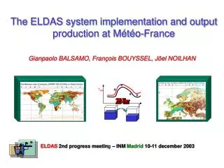
T2m t The ELDAS system implementation and output production at Météo-France Gianpaolo BALSAMO, François BOUYSSEL, Jöel NOILHAN 2D-Var ELDAS 2nd progress meeting– INMMadrid10-11 december 2003
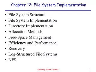
Plan of the presentation • ELDAS at Météo-France • The implementation of the system • The NWP model (ARPEGE) • The coupling to atmosphere (Blending) • The data Assimilation technique (Simplified 2D-VAR) • VALIDATION OF ECOCLIMAP & 2D-VAR • May-June 2003 • Comparison of ALADIN and ARPEGE on June 2000 • 2000/2003 comparison SWI and NDVI anomaly • ELDAS EXPERIMENTS • May-June 2000 without precipitation forcings • ELDAS FORCINGS • Use of precipitation forcing • May-June 2000 with precipitation forcings
Mahfouf (1991), Callies et al. (1998), Rhodin et al. (1999), Bouyssel et al. (2000), Hess (2001), Balsamo et al. (2003) Formalism: T2m t RH2m t Wp t 6-h 12-h 18-h 0-h Variational surface analysis J(x) = J b(x) + J o(x) = ½ (x – xb) TB-1 (x – xb) + ½(y – H(x))TR-1 (y – H(x)) Continuous analysis x is the control variables vector y is the observation vector H is the observation operator The analysis is obtained by the minimization of the cost functionJ(x) is the background error covariance matrix B is the observation error covariance matrix R • Advantages:Easier assim. asynop. obs. Extension on longer assim. Window (24-h)
ARPEGE:Global spectral stretched model 20 to 200 km, 41 levels (1 hPa) , 6h assimilation cycle for Surface Variables Atmospheric Blending (to avoid full re-analysis) The NWP model and the ELDAS resolution Cycle 25t1_op3 Operational version of May 2003 (stretching factor 3.5 )
+6hfcst +6hfcst +6hfcst +6hfcst The land surface analysis OI New T2m, Rh2m, Ts, Tp, Ws 2D-Var New Wp The atmospheric coupling • The atmospheric state is not re-analysed but a « Blending » technique is used to save atmospheric feedback of new land surface state
Archive AtmosphericAnalyse Atmosphericguess Atmosphericguess +6hfcst New Land Surface Analysis The atmospheric coupling Restore Blending Archive AtmosphericAnalyse « + » New Land SurfaceAnalysis New Land SurfaceAnalysis
Plan of the presentation • ELDAS at Météo-France • The implementation of the system • The NWP model (ARPEGE) • The coupling to atmosphere (Blending) • The data Assimilation technique (Simplified 2D-VAR) • VALIDATION OF ECOCLIMAP & 2D-VAR • May-June 2003 • Comparison of ALADIN and ARPEGE on June 2000 • 2000/2003 comparison SWI and NDVI anomaly • ELDAS EXPERIMENTS • May-June 2000 without precipitation forcings • ELDAS FORCINGS • Use of precipitation forcing • May-June 2000 with precipitation forcings
2D-Var + Ope OI + Ope OI + Eco 2D-Var + Eco The experimental frame Improved OI for Wp Operational Physiography Improved OI for Wp Ecoclimap Physiography Simplified 2D-VAR for Wp Operational Physiography Simplified 2D-VAR for Wp Ecoclimap Physiography
2D-Var + Ope OI + Ope OI + Eco 2D-Var + Eco
2D-Var + Ope OI + Ope OI + Eco 2D-Var + Eco
1 month score evolution (T2m RH2m RMSE(P6-A)) OO Utc 12 Utc O6 Utc 18 Utc
Comparison of large scale soil moisture with satellite derived soil moisture (TRMM) Using Backscattering Coefficient of TRMM Precipitation RadarSeto et al. 2003(submitted to J. of Geo. Res.)
Plan of the presentation • ELDAS at Météo-France • The implementation of the system • The NWP model (ARPEGE) • The coupling to atmosphere (Blending) • The data Assimilation technique (Simplified 2D-VAR) • VALIDATION OF ECOCLIMAP & 2D-VAR • May-June 2003 • Comparison of ALADIN and ARPEGE on June 2000 • 2000/2003 comparison SWI and NDVI anomaly • ELDAS EXPERIMENTS • May-June 2000 without precipitation forcings • ELDAS FORCINGS • Use of precipitation forcing • May-June 2000 with precipitation forcings
Consistency of results over June 2000: I) ALADIN The results obtained with a 2D-VAR assimilation cycle within ALADIN LAM model provided a more realistic soil moisture field compared to the hydrological coupled model, SAFRAN-ISBA-MODCOU (forced by Prec., Rad.) Balsamo et al. (2003) Habets et al. (2003)
Consistency of results over June 2000: II) ARPEGE The same comparison is produced for the ELDAS soil moisture obtained with the ARPEGE model. An improved ELDAS cycle (no precipitation) Habets et al. (2003)
June July +positive Index 2003/2002 +negative (CNES, 2003) Images SPOT/VEGETATION Variation of NDVI 2003 within respect to 2002 Drought of summer 2003: Comparison of soil moisture and NDVI anomaly On the 30 June 2003 (exp. 2D-Var + Ecoclimap (Masson et al. 2003)) Variation of SWI at 30 June 2003 compared to 30 June 2000 (ELDAS)
Comparison of large scale soil moisture variation and NDVI anomalies over Africa Variation of SWI at 30 June 2003 compared to 30 June 2000 (ELDAS)
+6hfcst +6hfcst +6hfcst +6hfcst Calculation of the 24-h ARPEGE accumulated precipitation and innovation The 2D-VAR cycle and the Precipitation readjustment • In order to fully benefit of the 2D-VAR analysis and the Precipitation readjustment the two steps are applied sequentially OI New T2m, Rh2m, Ts, Tp, Ws 2D-Var New Wp 00UTC 06UTC 12UTC 18UTC 00UTC 06UTC
Usage of ELDAS Precipitation forcings: I step Can we set a coefficient as Wpa - Wpf = aWpP24-h D P24-h
Usage of ELDAS Precipitation forcings: II step Guess Observation Obs-Guess
the two cycles without and with Precipitation readjustment are compared Usage of ELDAS Precipitation forcings: III step 2D-Var 2D-Var + p24h
the nearest point has been used for MF/INM interpolation and it is planned to be used also for the final production since it avoids post processing and save self consistency of surface fields. Interpolation to final ELDAS grid
Conclusions • Validation of simplified 2D-Var and ECOCLIMAP database for the summer 2003 with the ARPEGE GCM model • Comparison with results previously obtained with ALADIN-France over Europe. • Production (advance phase) of ELDAS output without and with precipitation forcing • Local archive at 1-h rate and preparation of interpolation/grib procedure for MARS archive.
Phase I 2D-VAR soil moisture analysison a 24-h window 24-h forecast Arpege GCM Atmospheric Restoreto the analysis Surface Update of the new 2D-VAR land surface variable
Phase II 2D-VAR soil moisture analysison a 24-h window 24-h forecast Arpege GCM Precipitation Obs. forcing Atmospheric Restore (or Blending) Surface Update of the new 2D-VAR land surface variable Grib and Archiveon MARS To do
? Perspectives 2D-VAR land surface analysison a 24-h window Heating rates Assimilation 24-h forecast Arpege GCM Rad. Prec Obs. forcing Atmospheric Restore (or Blending) Surface Update of the new 2D-VAR land surface variable(s) ? B matrix Update