Download
1 / 34
340 likes | 478 Views
What’s all this VLBI stuff, anyway?. Tom Clark NVI / NASA Goddard Space Flight Center mailto: K3IO@verizon.net _____________________________________________________________. IVS TOW Workshop Haystack – April 30, 2007. The Topics for Today:. Some Fundamentals of Radio Astronomy

E N D
What’s all this VLBI stuff, anyway? • Tom Clark NVI / NASA Goddard Space Flight Center mailto: K3IO@verizon.net _____________________________________________________________ IVS TOW Workshop Haystack – April 30, 2007 Haystack – April 30, 2007
The Topics for Today: • Some Fundamentals of Radio Astronomy • Noise, Temperature = Power • Janskys, Flux Density & Sensitivity • Some Fundamentals of Interferometry • What is an interferometer? • Resolution & Spatial Frequency • Heisenberg’s Uncertainty Principle • The U-V Plane and Aperture Synthesis • How is VLBI Different? • Breaking the Wires and shipping the bits • Quasars and similar beasties • Closure Phase • Group Delay Note: Some important concepts are marked like this Haystack – April 30, 2007
Some Simple Thermodynamics • Consider two isolated universes at two different temperatures, T1 & T2 , and let ∆T = T1-T2. • In each universe put either a resistor or an antenna and connect them with a perfect transmission line • If T1 > T2, then power P = 2k•∆T•B until the temperatures equalize. where k = Boltzman’s constant = 1.38 •10-23 watts/ºK/Hz Bandpass Filter BW = B T1 T2 Haystack – April 30, 2007
Power = Temperature [and the Mysterious factor of 2] • The receiver will see a delivered power P = k•T•B where the previous factor of 2 disappeared because the receiver only responds to half the noise signal. The noise has half it’s power in each of two orthogonal (i.e. sine vs cosine) components. A second receiver, with its LO shifted by 90º, would see the other, independent component which also has a power P = k•T•B Radio Receiver with detector bandwidth = B T Power Meter Haystack – April 30, 2007
Flux Density & Janskys • Flux Density is the measure of the amount of power falling on a 1 m2 surface area. • In radio astronomy, we measure the brightness of a radio source in Janskys: 1 Jansky = 1 Jy = 10-26 watts/m2/Hz • In geodesy, most sources of interest have fluxes of 0.1 – 10 Jy • A lot of high sensitivity astronomy is done on sources < 1 mJy (10-29 w/m2/Hz) Haystack – April 30, 2007
Sensitivity We saw earlier that a receiver will indicate the total power of P = k•T•B. Let’s now consider what temperature contributions are in T: TCMB = cosmic microwave background ~ 3ºK + TATM = atmosphere absorbs some of the signal + TLOSS = antenna ohmic losses + TSPILLOVER = antenna feed sees trees, ground, etc + TLNA = Low Noise Amplifier in receiver + TMISC = other miscellaneous contributions TSYS = the sum of all these contributions TSYS must be compared to TSOURCE = the small contribution from radio source that we want to see: S/N = TSOURCE/TSYS Haystack – April 30, 2007
Sensitivity cont’d • In radio astronomy, our signal is random noise. It can be shown that if we have noise with a Band-width B Hz, then we obtain a fresh, independent measurement of the noise every 1/B seconds. • Now add all these independent samples forseconds (called the integration time). • The total number of samples collected will ben = B • • Statistics tells us that the uncertainty of an average made up of n samples is ≈ 1/√n Haystack – April 30, 2007
Sensitivity cont’d • Therefore we see that our noise measurement will have an RMS noise level of TSYS • ρ √(B•) where ρ is a number typically in the range 1 to π depending on the specifics of the radiometer • To detect a source with good certainty, it is desirable to strive for TSOURCE > 5 δT • This is usually achieved by • Integrate Longer to increase √ • Build a new receiver with better TSYS • Use a bigger telescope δT ≈ Haystack – April 30, 2007
S (D/)●sin() D/ 1 2 The Basic 2-Element Interferometer Consider a 2 element interferometer with the elements separated by a distance D operating at a wavelength . Observe a distant source S at an angle . We bring the signals together & measure the phase = [2π(D/) ● sin()] by multiplying the two signals. Now let the source S move across the sky, changing the angle . The output of the multiplier (a.k.a. correlator) will be of the form: V() ~ cos() = cos[2π(D/) sin()] When the antenna is “broadside” with small we can use the approximation sin() and write Multiplier V() ~ cos [2π(D/) ● ] V() Haystack – April 30, 2007
The Concept of Spatial Frequencies • In the 2-element interferometer, we saw that the output is of the form V()~cos [2π(D/)●]. We have sinusoidal “fringes” on the sky with a periodicity of • Example: Consider 2 small antennas spaced 4.2 meters apart at 70 cm are spaced by a distance of 6 , and will exhibit interferometer fringes spaced 1/6 radians = 9.5˚. • This expression for V() is similar to the form of a cosine wave V(t)~cos(2πft). We define the (spatial) frequency as (D/) and its orthogonal domain as , the angle on the sky (measured in radians). An interferometer acts as a filter to isolate structure of the sky that has a periodicity of / D cycles/radian • If we have a complex pattern on the sky, then a series of baselines with different D/ can be used to decompose the brightness distribution of the source. This is the basis of Aperture Synthesiswhich is the basis of much of modern Radio Astronomy! ∆ (in radians) = / D Haystack – April 30, 2007
Two antennas separated by 6 1 Radian 1 2 3 4 5 6 Equally Spaced “Bread Slices” Spatial Frequency = D/ cycles/radian Haystack – April 30, 2007
Some Interferometer ExamplesInterferometer fringes for D=d●(1,2,4,8,16) Source = 5d/100 Radians Haystack – April 30, 2007
Resolution of source = 5●d/100 Radians Source = 5d/100 Radians Haystack – April 30, 2007
Resolution of source = 11●d/100 Radians Source = 11d/100 Radians Haystack – April 30, 2007
Resolution of source = 21●d/100Radians Source = 21d/100 Radians Haystack – April 30, 2007
Putting These Interferometers Together to make a One-Dimensional Visibility Function Points sampled for baselines D=d•(1,2,4,8,16) λ & sources of size (5,11,21) SINC(x) = sin(πx) (πx) Haystack – April 30, 2007
A 27-element Interferometer The VLA in New Mexico The VLA consists of 27 85’ telescopes in a “Y” shape spanning a total of nearly 40 km west of Socorro, NM.(Sometimes a 28th element 52 km west of the VLA at Pie Town, NM is added for more resolution) 27 elements yield (27)*(26)/2 = 351 simultaneous 2 element inter-ferometers. Haystack – April 30, 2007
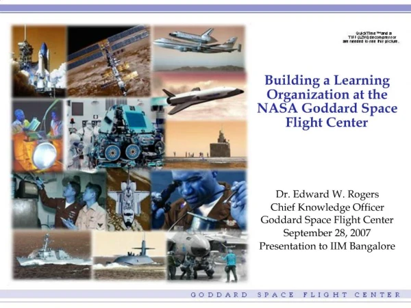
2-Dimensional Spatial Frequencies As the earth turns, the orientation of all 351 baselines rotate as seen from a source on the sky, synthesizing the equivalent of a ~40 km diameter dish: This example shows the equivalent Aperture Synthesis “dish” formed by observing a source at =45˚ for 12 hours. At the right, we see the “beam” formed by Fourier Transforming the U-V spatial coverage. Haystack – April 30, 2007
More VLA “u-v” Plane Coverage Haystack – April 30, 2007
Fourier Transforms and Antennas Just as frequency/time are related by a Fourier transform, the (voltage) distribution of signals across an antenna array is related to the (voltage) pattern of the antenna on the sky Ourearlier One-Dimensional interferometer example yielded a SINC(X) = visibility function. The Fourier Transform F {SINC(X)} is a “boxcar”, just like the d•(5,11,21)/100 model we assumed. Input Signal V(t) Aperture Illumination V(D/λ) Or 2D: V(u,v) Frequency (cycles/second) Spatial Frequency (cycles/radian) Or 2D: Image F sin(πx) (πx) Haystack – April 30, 2007
A Factoid to Remember If we have two domains that are related by a Fourier Transform like we just described: Input Signal V(t) Aperture Illumination V(D/λ) F Frequency (cycles/second) Spatial Frequency (cycles/radian) • If a “signal” is • in one domain, then it is in the other. • Big Antenna ―› Small Beamwidth • Wide Beamwidth ―› Small Antenna • Sharp Pulse ―› Wide RF Bandwidth Δf 1/t W I D E Narrow • ∆ (radians) = / D Haystack – April 30, 2007
Werner Heisenberg’sUncertainty Principle ! ! ! Haystack – April 30, 2007
The Uncertainty Principle in The Real World • What Schrödinger didn’t understand is that Quantum Mechanics is intimately related to Fourier Transforms. • One of the Heisenberg’s two expressions for the uncertainty principle is ∆E●∆t > h/2π , where Planck’s Constant h = 6.626x10⁻³⁴ Joule-seconds • We have learned that the change in Energy associated with an atomic transition between two levels ∆E is associated with the emission of a photon of frequency ∆f as ∆E = h ● ∆ f. • Substituting for ∆E & dividing by h, we get the equivalent expression for the Uncertainty Principle ∆f●∆t > 1/2π Haystack – April 30, 2007
Some implications of ∆f●∆t > 1/2πMeasuring Frequency with a Counter • If we measure the frequency of an oscillator with a counter, we count the number of cycles N that occur in a time ∆t as defined by a clock in the counter. • But because the ∆t window can start & end anywhere in the sine wave, we have an uncertainty in the measurement of ∆N=±[0-2] counts. By averaging several measurements, we can determine N±∆N to better than ±1 count. • The oscillator’s frequency is then determined to be f= (N±∆N) /∆t with an uncertainty ∆f ● ∆t ±1 count • If we had actually measured the phase of the at the start and end of the ∆t measurement, we could have achieved the Heisenberg limit ∆f ● ∆t 1/2π even if the S/N is poor. • If the (S/N) is improved and the phase is measured more accurately, then the uncertainty will become ∆f ● ∆t 1/[2π●(S/N)] Haystack – April 30, 2007
The Uncertainty Principle in Radio Astronomy • Interferometers have an antenna pattern with sinusoidal peaks spaced ∆=(/D) radians so measuring the position of a source to by counting fringes, we achieve a measurement precision of ●(D/) ±1 fringe (just like the frequency counter). • If the S/N is poor and we use fringe phase as the observable, then we reach the Uncertainty Principle limit of ● (D/)> 1/2π • If you have a reasonable (S/N), you can measure the phase of the sinusoidal fringe and infer the position with an uncertainty of fraction of a radian: (/D) ● (S/N)-1 ● 1/2π • For an intermediate VLA baseline (~8km) @ 15 GHz (=2cm) we have fringes spaced ∆=/D = 5x10⁻⁷ radians = ½ arcsecond and it should be possible to measure source positions to < .02arc sec, assuming all measurement errors (including atmospheric path delays) can be calibrated. • VLBI baselines as long as 12,000 km (Hawaii to South Africa) at =3.8 cm. (D~3x10⁸) yield fringes of ∆<1 milliarcsecond in size. Haystack – April 30, 2007
Properties of the Fourier Transform(or, Fourier's Song) Integrate your function times a complex exponential.It's really not so hard, you can do it with your pencil.And when you're done with this calculationYou've got a brand new function - the Fourier Transformation.What a prism does to sunlight, what the ear does to sound,Fourier does to signals, it's the coolest trick around.Now filtering is easy, you don't need to convolve;all you do is multiply in order to solve. ------------------------------------------ From time into frequency --- from frequency to time ------------------------------------------ Every operation in the time domain, has a Fourier analog - that's what I claim. Think of a delay, a simple shift in time – It becomes a phase rotation - now that's truly sublime!And to differentiate, here's a simple trick,just multiply by j omega, ain't that slick?Integration is the inverse, what you gonna do?Divide instead of multiply - you can do it too. ----------------------------------------------- From time into frequency --- from frequency to time --------------------------------------------- Let's do some examples... consider a sine.It's mapped to a delta, in frequency - not in time.Now take that same delta as a function of time,Mapped into frequency - of course - it's just a sine! Sine x on x is handy, let's call it a sinc.Its Fourier Transform is simpler than you think.You get a pulse that's shaped just like a top hat...Squeeze the pulse thin, and the sinc grows fat.Or make the pulse wide, and the sinc grows dense,The uncertainty principle is just common sense. – Stolen from Bill Sethares @ http://eceserv0.ece.wisc.edu/~sethares/mp3s/fourier.html Haystack – April 30, 2007
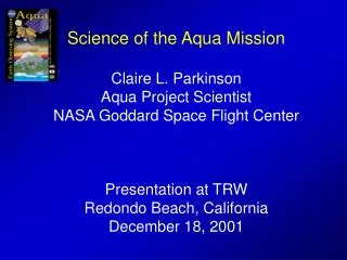
Quasars and other beasties • In the mid 1960’s it was noted that some “radio stars” were variable on time scales ~weeks to months. It is hard to envision any source that is larger than ~1 light-month in size that can vary that rapidly. • For one of these “quasars” (3C273), old photographic plates (like from 1929) tell that the optical “star” is also variable. • If we assume that these object are extragalactic, then the sources must have sizes and/or structure measured in milliarcseconds (i.e. ~10-8 radians). • If the sources are this small and this far away, then the equivalent brightness temperatures must be ~ 1014 to 1015 ºK !!! Haystack – April 30, 2007
Quasars and other beasties • In order to measure the size a source 10-8 radians in size, we need a baseline ≥ 108λ. • At a wavelength λ = 10cm, this requires baselines ≥ 107m = 104 km 6000 miles. • [an aside: The meter was originally defined as 10-7 times the distance from pole to equator along the meridian of Paris. This leads to the circumference of the earth ≈ 40,000 km and the radius of the earth ≈ 40,000/2π = 6370 km] • In 1967, groups in the US and Canada succeeded in breaking the 1000 km barrier using atomic clocks and tape recorders. • US = Mark-1 with 800 BPI 7-track computer tape (360 kHz, 720 kb/s, with one tape lasting 3 minutes): Greenbank-Arecibo = 2550 km @ 610MHz = 5.2 Megaλ => 38 milliarcsec fringes. • Canada = Analog studio video tape recorders (4 Mhz): Algonquin-Penticton = 3074 km @ 448 MHz = 4.6 Megaλ => 44 milliarcsec fringes. • After about 1968, all systems migrated to digital recording using Computer Tape (Mk1 & DSN), Video Tape (Mk2, Canada, Japan), Instrumentation Tape (Mk3 & 4) and now RAID-like Computer Disk Arrays. • By 1971 well-sampled visibility curves of 3C279 showed a well defined double source • Haystack-Goldstone baseline @ λ=3.8 cm (100 Megaλ => 2 milliarcsec fringes. • These measurements were repeated a few months later and showed apparent superluminal motion ( velocity ≈ 10c). Haystack – April 30, 2007
Galactic & Solar System Objects • Also in 1967 (with Mark-1) were the first observations of OH Masers at 1665-1667 MHz (λ = 18 cm). These objects exhibit numerous small, narrow bandwidth “hot spots”. • Later, other Maser sources associated with methanol, H2O, SiO, NH3 and other chemicals have been detected. • At frequencies below ~ 1 GHz pulsars have proven interesting. • The planet Jupiter radiates “bursts” at frequencies below 38MHz. VLBI on Jupiter dates back to the early 1960’s, predating the Quasar VLBI! • Interplanetary spacecraft have been tracked with VLBI, using differential measurements between the spacecraft and quasars for navigation. • The Apollo “Lunar Rover” was tracked (λ = 13 cm) with respect to the LEM “home base”. Haystack – April 30, 2007
Phase in Interferometry • We noted earlier that the image of a source observed by an interferometer array can be related to the observed visibility function via a Fourier transform. What’s the sign ? - or + • This assumes that each data point is a complex phase (& sign) and amplitude. • In VLBI, we have independent phase/frequency standards (H-masers), so we have lost track of the absolute RF signal phase Haystack – April 30, 2007
Phase in VLBI (1) VLBI people have come up with 3 main ways to solve the undefined phase dilemma: • Rapidly switch between the source of interest and a nearby “point” source. Then do the mapping W.R.T. the reference source. The sources need to be close enough so that phase errors caused by the atmosphere are the same. • If you are really lucky, the reference source is in the same telescope field of view. This has been used extensively for mapping of OH, H20 etc. maser sources. • The switching needs to be fast enough so that phase drifts in the H-Maser and atmosphere are small. Haystack – April 30, 2007
Phase in VLBI (2) • If we observe a source with 3 (or more) stations with different baselines, then we can use “closure phase”. • If the source is symmetric then the 3 observed phases ΦAB + ΦBC + ΦCA = 0. • If the source is not symmetric (like a core+jet), then the triplet phase ≠ 0. • Models containing the observed closure phases and amplitudes can be “observed” in the computer and iterated until the observations from the model match the data. • Then the paper is sent to Ap.J. Haystack – April 30, 2007
Phase in VLBI (3) • Especially for Geodesy and Astrometry, the principal observation type is called the “Group Delay” = G = ΔΦf/Δf. • Usually, fringe phase Φf is measured in a series of separated, narrow bands (at IF) that cover a wider “spanned bandwidth” in a technique named “bandwidth synthesis”. A common example is the use of 8 IF channels at X-band spanning more than 700 MHz. • We earlier saw that the Uncertainty Principle predicts ∆f ● ∆t 1/[2π●(S/N)].Therefore a spanned bandwidth Δf~500 MHz & S/N~30 would have an RMS uncertainty ~11 picoseconds. Haystack – April 30, 2007
FINIS Thank you for participating in this marathon! Any Questions (or are you ready for coffee?) Haystack – April 30, 2007