3.7 Example: Bioassay experiment
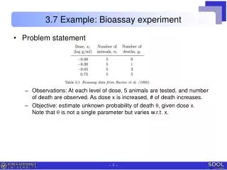
3.7 Example: Bioassay experiment. Problem statement Observations: At each level of dose, 5 animals are tested, and number of death are observed. As dose x is increased, # of death increases.

3.7 Example: Bioassay experiment
E N D
Presentation Transcript
3.7 Example: Bioassay experiment • Problemstatement • Observations: At each level of dose, 5 animals are tested, and number of death are observed. As dose x is increased, # of death increases. • Objective: estimate unknown probability of death q, given dose x. Note that qis not a single parameter but varies w.r.t. x.
Establishing posterior distribution • Binomial distribution • Let the unknown death probability be ifor xi for ith group. • Then the data yi are binomially distributed: • Modeling dose response relation • is not constant but a function of dose x. Simplest trial is linear function. • This model has flaw that for very low or high x, it approaches ±∞.To meet this condition, introduce logistic transformation Then leads to • Relation is changed to This is called a logistic regression model.
Establishing posterior distribution • The likelihood • Likelihood of each individual group • Remark: model is characterized by two parameters , , not .Hence, these are the parameters to be estimated. • Joint posterior pdf • Prior distribution is assumed uniform or non-informative, i.e., • Remark: can we write down the expression in closed form ?Never seen the pdf like this, nor are there standard pdfs available.Nevertheless, this is probability distribution indeed.
Analyzing posterior distribution • Rough estimate of the parameters • We can crudely estimate these by least squares minimization (linear regression) of zi on xi where i=1,…,4. The solution for (, ) are (0.1,2.9). • We can also estimate standard error of (, ) The solution for (V, V) are (0.3, 0.5). • This gives us rough range of the parameters. ~ 0.1 ± 3*0.3 and ~ 2.9 ± 3*0.5
Analyzing posterior distribution • Contour or 3-D plot of joint posterior density • Define the domain as mean ± 3 std errors, which are [0.10.9]=[-1,1] x [2.91.5]=[1,5] . • Use computer program to plot contour, and find out the range is wrong indicating that the crude estimation was really crude indeed. • After trial & error, find out much wider range is needed, [-5,10]x[-10,40]. • Remarks • How can we analyze this distribution ?i.e., how can we get the mean, variance, confidence intervals, etc ?
Sampling from posterior distribution • Grid method (inverse cdf method) • Refer section 1.9 of Gelman or 9.2.3 of Mahadevan. • Procedure • In order to generate samples following pdf f(v), • Construct cdf F(v) which is the integral of f(v). • Draw random value U from the uniform distribution on [0,1]. • let v=F-1(U). Then the value v will be a random draw from f(v). • Practice • Generate samples for N(0.1). • Validate with analytic solution by comparing pdf shapemean, std, 95% conf bounds.
Sampling from posterior distribution • Factorization approach • Sample the two parameters a & b in the same way as the two parameters of normal distribution. where p(a|y): marginal pdf of a which is obtained by integration.p(b|a,y): conditional pdf of b given a. • Procedure • Normalize the discrete joint pdf, i.e., make the total probability value 1. • Make marginal pdf p(a|y) by simply summing over b. • Draw a from marginal pdf of a using grid method. • Draw b from conditional pdf of b|a. • Post-analyze using the samples: As we have obtained samples of a & b, one can evaluate several characteristics.
Sampling from posterior distribution • Sample results • Scatter plot & comparison with contour plot • Posterior distribution of LD50, which is the dose level x at which the prob. death is 0.5. Simulating this is trivial.
Posterior prediction by sampling • Original definition • In this problem, probability of death is predicted at a dose level x. • Practical solution • For each sample a & b, generate new y (which is prob. death q here). • By this way, simulation is much more convenient than the analytic (or numerical) integration.
Remarks on grid based method • Remarks • There can be difficulty finding correct location & scale for the grid points.If the area is too small, it can miss the important area.If the area is too large, it can miss the importance due to large interval. • When computing posterior pdf, overflow / underflow encountered usually because it is multiplication of individual pdfs.To avoid, introduce log to the posterior density. • Computation grow prohibitly as more parameters are included.500 grid for a parameter leads to 500^4 = 6.25e10 numbers for the whole grid, at which the function value should be evaluated. Conclusion: this method is not used in practice.