Download

1 / 46
460 likes | 635 Views
Adjust Survey Response Distributions Using Multiple Imputation: A Simulation with External Validation Frank Liu & Yu-Sung Su. We Want a Better Guess of Respondents' Preferences. How to Utilize M ultiple I mputation to make better guesses about the respondent’s preferences?.

E N D
Adjust Survey Response Distributions Using Multiple Imputation: A Simulation with External Validation Frank Liu & Yu-Sung Su
How to Utilize Multiple Imputation to make better guesses about the respondent’s preferences?
Calculating proportions based on raw data and omitting the non-response data result in biased proportion of interested variables (Bernhagen & Marsh, 2007). • Multiple Imputation (MI) is a cost-efficient and methodological sound approach for better use of raw survey and poll data (Barzi, 2004).
Picture Source: Kyle F. Edwards, Christopher A. Klausmeier, and Elena Litchman (2011)
While most studies use MI for modeling, there is room to examine to which MI can be applied to electoral forecast (King et al., 2001; Snijders & Bosker, 2011).
Joint MI (Amelia II) vs. Conditional MI (mi & MICE)
Joint MI assumes a multivariate normal distribution. vs. Conditional MI does NOT.
mi takes advantage of existing regression models to handle various kinds of variables types (Su, Gelman, Hill, & Yajima, 2011): • using a logistical regression model to predict a binary outcome, • Using an ordered logit regression model to predict an ordinal outcome, • Using a multinomial logit regression model to predict an unordered categorical outcome.
mi results can be very biased when data include extreme values (He and Raghunathan, 2009)
Data RDD telephone survey data about Taiwanese voters’ national identification (N=1,078), collected from Jan. 23 to Feb. 4, 2013. (AAPOR #3: 21.56%)
Study 1: Check Missingness Patterns • Using conditional MI algorithm to check its missingness patterns and to conduct MI. • the data should be at least missing at random (MAR), i.e., the missingness mechanism does not depend on the unobserved data. • MCAR > MAR > MNAR
Check the Missingness Patterns 1: Specify a conditional MI model • include many valid auxiliary variables (17); 2: Contrast Simulated Data with MI Data • Set the imputed datasets as the baseline for comparison • create three copies of the MI data • randomly remove values from the completely imputed data according to the original missing rate of the data, i.e., 61%.
We create simulated datasets by modeling the missingness of each variable conditional on a linear combination of the rest of variables with logistic regressions. • Then we use the predictive missingness to create missing values on the three imputed data. • In short, we compare simulated datasets with the original MI dataset.
Results of the Check for MCAR (2) • Table 2: • Summary of the camp variable between the original data and imputed MCAR datasets. Note: + The mean’s and SE’s reported here are pooled mean and SE’s for three chains of MI.
Results of the Check for MCAR (3) Figure 3: Plots of Camp Variable against Other Variable Using the Imputed MCAR data.
Results of the Check for MAR (2) • Table 3: • Summary of the camp variable between the original data and imputed MAR datasets. Note: + The mean’s and SE’s reported here are pooled mean and SE’s for three chains of MI.
Study 2: External Validation • 1: compare respondents' answers with MI guesses • figure out how well the MI prediction works • 2: understand why prediction performs not so well, if this is the case. • follow-up telephone surveys with identity check • Face-to-face one-by-one interviews for explanations
Follow-up telephone surveys • Called out • for the 658 respondents’ camp identification whose political camp id is NA. (April 13-15, 2013) • Forced to choose between Green and Blue. • N=143 • Identity check • Answers must be consistent with the first survey regarding two questions: (1) whether ever going to mainland China in the past two years; (2) the frequency of watching political news
3. In-depth Interview: • 45 out of 143 respondents were contacted for face-to-face one-by-one Interview. (incentive: cash $70) • 5 out of 45 respondents were interviewed between April 20 to May 6, 2013.
Findings the total number of the 145 respondents whose values fall between .45 and .55: 19
Summary • These “danglers” are politically aware. • Explanations for the ambivalence: • potential blue camp supporters (ID 905, 206, 384, and 286) have become unsatisfied with the incumbent's performance and public policy. • potential green camp supporters (ID 905, 206, 384, and 286) are affected by nationalism. • Cross-pressured (ID 140, 384, and 286).
Conclusion • MI scores reflect respondents’ partisan orientation, including the level of their ambivalence. It seems reasonable to adopt this method to reconstruct the distribution of partisan orientation of the electorate. • By face-to-face interviews inconsistency of their answers can be explained.
Implications & Suggestions • Encourage respondents to give up answering those they could not answer • Explore auxiliary questions for partisanship (e.g., policy and performance ones) and encourage respondents to answer sincerely that seem less sensitive to them. • Use these easier auxiliary variables for MI.
Continue to test the reliability of this method using panel data. • Be aware of the limit of forcing respondents to choose an answer. Alternative methods or question wording of probing true answers about partisanship are still needed.
Thank you. request for the paper, data, and/or R code frankcsliu@gmail.com