Download
1 / 42
550 likes | 877 Views
Drude’s Classical Model of Metallic Conduction Contrasted with Sommerfeld’s Quantum Mechanical Theory. Drude’s Classical Model of Metals (Beautifully explained in depth in Ashcroft and Mermin , Ch. 1)

E N D
Drude’s Classical Model of Metallic ConductionContrasted withSommerfeld’s Quantum Mechanical Theory
Drude’s Classical Model of Metals • (Beautifully explained in depth in Ashcroft and Mermin, Ch. 1) • Modern condensed matter physicswas BORNwiththe discovery of the electronby J.J. Thompson in 1897. • Soon afterwards (1900) Drude used the new concept to postulate • A theory of metallic conductivity
Drude’s Assumptions • 1. Matter consists of light negatively charged electrons which are mobile, & heavy, static, positively charged ions. • 2. The only interactions are electron-ion collisions, which take place in a very short time t. • The neglect of the electron-electron interactions is • The Independent Electron Approximation. • The neglect of the electron-ion interactions is • The Free Electron Approximation.
The mean time between collisions is t. Ion Trajectory of a mobile electron Drude’s AssumptionsContinued 3. Electron-ion collisions are assumed to dominate. These will abruptly alter the electron velocity & maintain thermal equilibrium. 4. The probability of an electron suffering a collision in a short time dt is dt/τ, where 1/τThe Electron Scattering Rate. Electrons emerge from each collision with both the direction & magnitude of their velocity changed; the magnitude is changed due to the local temperature at the collision point.1/t is often an adjustable parameter. See the figure.
Drude Conductivity: Ohm’s “Law” V = IR • The ResistanceR is a property of a conductor (e.g. a wire) which depends on its dimensions, V is a voltage drop & I is a current. • In microscopic physics, it is more common to express Ohm’s “Law”in terms of a dimension-independent conductivity (or resistivity) which is intrinsic to the materialthe wire is made from. • In this notation, Ohm’s “Law” is written • E = rjorj = sE(1) • E = Electric Field, j =Current Density, • r =The resistivity & s =The conductivityof the material. • Consider a wire of cross sectional area A, with a current flowing in it. The current consists of n electrons per unit volume, all moving in the direction of the current with velocity v: • The number of electrons crossing area A in time dt is nAvdt j A
The charge crossing A in dt is -nevAdt, so j = -nev. (2) In the real material, we expect the electrons to be moving randomly even in zero electric field due to thermal energy. However, they will have an average, or drift velocityalong the field direction. vdrift = -eEt / m(3) This comes from integrating Newton’s 2nd Law over time t. This is the velocity that must be related to j. Combining (2) & (3) gives j = (ne2t / m)E. Comparison of this with j = sE gives the Drude conductivity:
As is often true for physics models, this result for • σ has been obtained using some very simple • assumptions, which surely cannot be correct in • reality! How can this result be tested? • First ask: Does the Drude assumption of • scattering from ions seem reasonable? • Check it experimentally by measuring s • for a series of known metals, and, using sensible • estimates for n, eand m, estimatet. • Results show that,at least for “simple metals” • t 10-14s at room temperature.
For many cases, instead of a an average • scattering time t, it’s often necessary to • formulate a theory of conductivity in terms of • An average distance between collisions. • This distance is called • The mean free path between collisions. • To do this, we have to consider the average • electron velocity. This should not be vdrift, which • is the electron velocity due to the electric field. • Instead, it should be vrandom, the velocity • associated with the intrinsic thermal energy of • the electrons.
Lets estimate vrandom by treating the electrons as a classical ideal gas and using the result from classical statistical physics: The Equipartition Theorem ½(m)v2random = (3/2)(kB)T (For a simple derivation, see any Physics I textbook!) Results: The mean free path is l = vrandomt 1-10 Å This is of the order of interatomic distances, so it is reasonable!
ΔV j jq -ΔT A Very Important Experimental Result for Metals: “The Wiedemann-Franz Law” Since 1853, it has been known that one of the most universal properties of metals is an experimentally well verified relationship between the thermal and the electrical conductivities. As we just discussed, in the presence of an external electric fieldE, the current density j is given by Ohm’s “Law”: j = sE In simple one dimensional geometry as in the figure, j = sE = sdV/dx The thermal analogue of this is jq = -kdT/dx. k Thermal Conductivity.
Drude’s assumption was that k in metals is dominated by the electronic contribution. A result from elementary kinetic theory is: k = (1/3)vrandomlcel (4) where cel is the electronic specific heat per unit volume. Each electron has an energy (3/2)kBTso, for n electrons per unit volume: Etot = (3/2)kBT, cel = dEtot/dT = (3/2) nkBT Recall that l = vrandomt, & divide k by σ = (ne2t / m) giving:
Dividing by T gives the simple result that This is a very nice result!! All the parameters that might be regarded in some way as poorly known have dropped out, leaving what looks like it might be a universal quantity. Experimentally, this is indeed the case. The measured number is a factor of two different from this Drude result, but in his original work, a numerical error made the agreement appear to be exact!
So, Drude’s model appeared to be reasonably self-consistent in identifying electron-ion collisions as the main scattering mechanism, and had a triumph regarding the most universal known property of metals. This was enough to set it up as the main theory of metals for two decades. However, fundamental problems began to emerge: 1. It could not explain the observation of positive Hall coefficients in many metals (discussed later). 2. As more became known about metals at low temperatures, it was obvious that since the conductivity increased sharply, l was far too long to be explained by simple electron-ion scattering. 3. A vital part of the thermal conductivity analysis is the use of the kinetic theory value of 3/2nkB for the electronic specific heat. Measurements gave no evidence for a contribution of this size.
The solution to these issues and the other unpleasant difficulties like the existence of insulators would not have come in a thousand years of hard work, if we had been restricted to classical physics. “The physics of solids is deeply quantum mechanical; indeed condensed matter is arguably the best ‘laboratory’ for studying subtle quantum mechanical effects in the 21st century.” Advanced general interest reading on this issue (probably more suitable some time later in the year unless you have already read quite a bit about quantum mechanics): ‘The theory of everything’, R.B. Laughlin and D. Pines, Proc. Nat. Acad. Sci. 97, 28 (2000).
Summerfeld’s Quantum Mechanical Model of Electron Conduction in Metals The Free Electron Gas A Non-trivial Quantum Fluid Bohr, de Broglie, Schrödinger, Heisenberg, Pauli, Fermi, Dirac….. With the development of quantum mechanics, a natural step was to formulate a quantum theory of electrons in metals. This was first done by Sommerfeld. Assumptions Most are very similar to those of Drude. Free & independent electrons, but no assumptions about the nature of the scattering. Starting point: time-independent Schrödinger equation
Note that no other potential terms are included; hence we can solve for a single, independentelectron and then investigate the consequences of putting in many electrons. To solve the Schrödinger equation we need appropriate boundary conditionsfor a metal. Standard ‘particle in a box’: set ψ = 0 at boundaries. This is not a good representation of a solid, however. 1. It says that the surface is important in determining the physical properties, which is known not to be the case. 2. It implies that the surfaces of a large but not infinite sample are perfectly reflecting for electrons, which would make it impossible to probe the metallic state by, for example, passing a current through it.
The most appropriate boundary condition for solid state physics is the periodic boundary condition: , p integer, etc. (9) Consider a cube of side L for mathematical convenience; a different choice of sample shape would have no physical consequence at the end of the calculation. Solving then gives allowed wavefunctions: Here V = L3 and the V-1/2 factor ensures that normalisation is correct, i.e. that the probability of finding the electron somewhere in the cube is 1.
(10) First, note energy eigenvalues: Then, note that yk is also an eigenstate of the momentum operator , with eigenvalue p = hk. Then we see the close analogy with a well-known classical result: (11) What is the physical meaning of these eigenstates? The state yk is just the de Broglie formulation of a free particle! It has a definite momentum hk.
It thus also has a velocity v = hk/m. How does the spectrum of allowed states look? Cubic grid of points in k-space, separated by 2p/L; volume per point (2p/L)3. We have just done a quantum calculation of a free particle spectrum, and seen close analogies with that of classical free particles. Answer: now we have to consider how to populate these states with a macroscopic number of electrons, subject to the rules of quantum mechanics. Sommerfeld’s great contribution: to apply Pauli’s exclusion principle to the states of this system, not just to an individual atom.
Result: At T = 0, get a sudden demarkation between filled and empty states, which (for large N), has the geometry of a sphere. ky State volume (2p/L)3 Fermi wavenumber kF . . . . . . . . . . . . kz kx Filled states State separation 2p/L Empty states Fermi surface Each k state can hold only two electrons (spin up and down). Make up the ground (T = 0) state by filling the grid so as to minimise its total energy.
We set out to do a quantum Drude model, and did not explicitly include any direct interactions due to the Coulomb force, but we ended up with something very different.The Pauli principle plays the role of a quantum mechanical particle-particle interaction The quantum-mechanical ‘free electron gas’ is a non-trivial quantum fluid! . Is everything OK here - doesn’t kF appear to depend on the arbitrary cube size L? (12) No - Quantities of interest depend on the carrier number per unit volume; the sample dimensions drop out neatly.
Calculate numerical values for the parameters. Use potassium Result: kF 0.75 Å-1 vF 1 x 10⁶ ms-1 F 2 eV How can we scale these quantum mechanical effects against something we are more familiar with? TF 25000 K ( recall kBT at room T 1/40 eV) This is a huge effect: zero point motion so large that a Drude gas of electrons would have to be at 25000 K for the electrons to have this much energy!
b) The T = 0 state occupation function. e Probability of state occupation 1 0 k kF e, k eF orkF A couple of much-used graphs relating to the Sommerfeld model: a) The free electron dispersion
The T=0 occupation discussed previously is a limit of the Fermi-Dirac distribution function for fermions: where the chemical potential m eF. (13) At finite T: ~ 2kBT f(e) m eF e The specific heat of the quantum fermion gas As expected, T is a minor player when it comes to changing things.
(14) The Fermi function gives us the probability of a state of energy e being occupied. To proceed to a calculation of the specific heat, we need to know the number of states per unit volume of a given energy ethat are occupied per unit energy range at a given T. Then internal energy Etot(T) can be calculated from (15) and the specific heat cel from dEtot/dTas before. Our next task, then, is to derive a quantity of high and general importance, the density of states g(e).
ky State volume (2p/L)3 dk . . . . . . . . . . . . kz kx State separation 2p/L Number of allowed statesper unit volume per shell thickness dk: spin
(16a, b) (17) Convert to density of states per unit volume per unit e (the quantity usually meant by the loose term ‘density of states’): Very important result, but note that e dependence is different for different dimension (see tutorial question 5).
g(e) n(e,T) Movement of electrons in energy at finite T eF e 2kBT (18) Evaluating integral (15) is complicated due to the slight movement of the chemical potential m with T (see Hook and Hall and for details Ashcroft and Mermin). However, we can ignore the subtleties and give an approximate treatment for eF >> kBT: [Etot(T) - Etot(0)]/V 1/2g(eF). kBT.2kBT = g(eF). (kBT)2
Differentiating with respect to T gives our estimate of the specific heat capacity: cel = 2g(eF). kB2T (19) The exact calculation gives the important general result that cel = (p2/3)g(eF). kB2T (20) c.f. Drude: How does this compare with the classical prediction of the Drude model? Combining g(eF) from (17) with the expression for eF derived in tutorial question 4 gives, after a little rearrangement (do this for yourselves as an exercise): (21)
A remarkable result:Even though our quantum mechanical interaction leads to highly energetic states at eF, it also gives a system that is easy to heat, because you can only excite a highly restricted number of states by applying energy kBT. The quantum fermion gas is in some senses like a rigid fluid, and its thermal properties are defined by the behavior of its excitations.
What about the response to external fields or temperature gradients? To treat these simply, should introduce another vital and wide-ranging concept, the Semi-Classical Effective Model. Faced with wave-particle duality and a natural tendency to be more comfortable thinking of particles, physicists often adopt effective models in which quantum behaviour is conceptualised in terms of ‘classical’ particles obeying rules modified by the true quantum situation. In this case, the procedure is to think in terms of wave packets centered on each k state as particles. Each particle is classified by a k label and a velocity v. Velocity is given by the group velocity of the wave packet: v = dw/dk = h-1de/dk = hk/m for free particles like those we are concerned with at present.
In the absence of scattering, we then use the following ‘classical’ equation of motion in applied E and/or B fields: mdv/dt = hdk/dt= -eE - ev B Assumption of the above: we cannot localise our ‘particles’ to better than about 10 lattice spacings. The uncertainty principle tells us that if we try to do that, we would have to use states more than 10% of our full available range (defined roughly by kF). Not, however, a particularly heavy restriction, since it is unlikely that we would want to apply external fields which vary on such a short length scale. This equation would produce continuous acceleration, which we know cannot occur in the presence of scattering.
Include scattering by modifying (22) to m(dv/dt + v/t) = -eE - ev B This is just the equation of motion for classical particles subject to ‘damped acceleration’. If the fields are turned off, the velocity that they have acquired will decay away exponentially to zero. This reveals their ‘conjuring trick’. The physical meaning of v in (23) must therefore be the ‘extra’ or ‘drift’ velocity that the particles acquire due to the external fields, not the group velocity that they introduced in their (3.22). In fact, this is formally identical to the process that we discussed in deriving equation (3) when we discussed the Drude model! It is no surprise, then, that it leads to the same expression for the electrical conductivity:
Following the procedure from Kittel gives us the Drude expression (3): Set B to zero and stress that the relevant velocity is vdrift; (23) becomes m(dvdrift/dt + vdrift/t) = -eE Steady state solution (dvdrift/dt = 0) is just vdrift = -(et/m)E If you give this some thought, it should concern you. What happened to our new quantum picture?
ky kz kx dk = h-1mvdrift= -eEτ/h To understand, consider physical meaning of the process: ky kz kx E = 0 Fermi surface is shifted along the kx axis by an E field along x. The ‘quasi-Drude’ derivation assumes that every electron state in the sphere is shifted by dk. This is ‘mathematically correct’, but physically entirely the wrong picture.
Which states can ‘interact with the outside world’? ky kz kx dk # of states (1/2 FS area) mom. gain # of states mom. gain x comp. only In the quantum model, only those within kBT of eF, i.e. those very near the Fermi surface. Pauli principle: only those states can scatter, so only processes involving them can relax the Fermi surface. So how does the ‘wrong’ picture work out? Consider amount of extra velocity/momentum acquired in equilibrium: Drude-like picture: Quantum picture: (24)
So the two pictures, one of which is conceptually incorrect, give the same answer, because of a cancellation between a large number of particles acquiring a small extra velocity and a small number of particles acquiring a large extra velocity. However, this is only the case for a sphere. As we shall see later, Fermi surfaces in solids are not always spherical. In this case, the Drude-like picture is simply wrong, and the conductivity must be calculated using a Fermi surface integral.
(25) What about thermal conductivity? Recall (4) from Drude model: k = 1/3vrandomlcel Here, vrandom can clearly be identified with vF, and l = vFt. Provided that t is the same for both electrical and thermal conduction (basically true at low temperatures but not at high temperatures; see Hook and Hall Ch. 3 after we have covered phonons), we can now revisit the Wiedemann-Franz law using (21) for the specific heat:
The approximate factor of two error from the Drude model has been corrected (p2/3 in quantum model cf. 3/2 in Drude model). Real question - how on earth was the Drude model so close? Answer: Because a severe overestimate of the electronic specific heat was cancelled by a severe underestimateof the characteristic random velocity. Thinking for the more committed (i.e. non-examinable): Would all quantum gas models give the same result for the Wiedemann-Franz law as the quantum fermion gas?
The modern conceptualisation of the quantum free electron gas: Make an analogy with quantum electrodynamics (QED). Thermal excitation: All particles with k kF, but sum over k = 0. Electrical excitation: All particles with k kF, but sum over k = 2 kF/3. ky ky kz kz kx dk Filled Fermi sea at T = 0 is inert, so it is the vacuum. Temperature and / or external fields excite special particle-antiparticle pairs. The role of the positron is played by the holes (vacancies in the filled sea with an effective positive charge). kx dk
Scorecard so far; achievements and failures of the quantum Fermi gas model 1. Successful prediction of basic thermal properties of metals. 2. Successful prediction of conductivity, as long as we don’t ask about the microscopic origins of the scattering time t - why is the mean free path so long in metals at low temperatures? What happened to electron-ion and electron-electron scattering? 3. Failure to predict a positive Hall coefficient. 4. No understanding whatever of insulators. ‘… So insulators, which cannot carry a current, must contain electrons too. In a metal they must be free to move, and in an insulator they must be stuck. I asked my tutor why this was so - and he told me that it was not understood. It was good to know the limits of knowledge at the time’ Quote from Sir Nevill Mott, writing about his time as a student in Cambridge, around 1925.
Quantum Sommerfeld gas: do wave mechanics and then think in an ‘equivalent particle’ picture Classical Drude gas Random velocity purely thermal: Random velocity dominantly quantum (due to Pauli principle): Specific heat cel = Large number of particles moving slowly. Small effective number of particles moving very fast, due to special quantum mechanical constraints.