Download
1 / 30
310 likes | 468 Views
Properties of Functions. A function, f , is defined as a rule which assigns each member of a set ‘A’ uniquely to a member of a set ‘B’. . A function f assigns exactly one value y to each x . We write y = f ( x ) or f : x y (‘ f maps x to y ’).

E N D
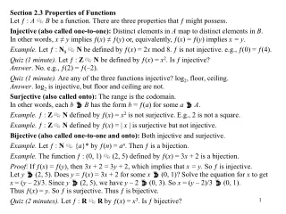
Properties of Functions A function, f, is defined as a rule which assigns each member of a set ‘A’ uniquely to a member of a set ‘B’. A function f assigns exactly one value y to each x. We write y = f (x) or f: x y (‘f maps x to y’). y is referred to as the image of x in f. Set ‘A’ is referred to as the Domain of the function and the set ‘B’ as the co-domain. The subset of ‘B’ which is the set of all images of the function is called the range of the function. It is possible for f (a) = f (b) and yet a≠ b. Often restrictions have to be placed on these sets to provide a suitable domain and range.
The modulus function The modulus or absolute value of x is denoted by | x | and is defined as Properties of |x| include:
Inverse functions The graph of and inverse function f-1 (x) is obtained by reflecting f (x) in the line y = x f-1 (x) is obtained by making x the subject of the formula. For example find the inverse function of f (x) = 2x +1
Placing restrictions on the domain and range can often ensure that a function has an inverse. When x < 1, f-1 (x) is undefined Hence largest suitable domain is x ≥ 1 giving a range y ≥ 0. The domain and range of the inverse function give us the range and domain respectively of the function.
Inverse Trig Functions Reflecting the curve in y = x. We need the largest region over which the curve is always increasing (or always decreasing).
Odd and Even Functions Even Functions Odd Functions Hence this is an even function. Hence this is an even function.
Hence this is an even function. Hence this is an odd function.
Page 100 Exercise 3 Questions 1(a), (e), (g), (h), 2(e), (c), (g), 3 Page 102 Exercise 4 Questions 1 and 2 Page 108 Exercise 8 Question 3.
Vertical asymptotes When h (a) = 0, the function is not defined at a.
(to the left of the line x = 1, the curve f (x) ∞-,negative infinity). (to the right of the line x = 1, the curve f (x) ∞+,positive infinity). The line x = 1, is called a vertical asymptote of the function. The function is said to approach the line x = 1 asymptotically.
Vertical asymptotes occur at x = -4 and x = -1. (-4 from the negative direction)
Page 109 Exercise 9 Question 1. TJ Exercise 1.
Non vertical asymptotes If g(x) is a linear function, it is known as either a horizontal asymptote or an oblique asymptote depending on the gradient of the line y = g(x). The behaviour of the function as x ∞+and as x ∞-can be considered for each particular case. (i) If the degree of the numerator < degree of the denominator, divide each term of the numerator and denominator by the highest power of x. (ii) If the degree of the numerator = degree of the denominator or the degree of the numerator > degree of the denominator, divide the numerator by the denominator.
The degree of the numerator = the degree of the denominator so we divide. 1 Hence y = 1 is a horizontal asymptote.
The degree of the numerator > the degree of the denominator so we divide. x +2 -1 Hence y = x + 2 is an oblique asymptote.
Page 110 Exercise 10 Questions 1(a), (b), (g), (f), (k), (l). TJ Exercise 2
1. Intercepts. • Where does the curve cut the y axis? x = 0 • Where does the curve cut the x axis? y = 0 2. Extras. • Where is the function increasing? f `(x) > 0 • Where is the function decreasing? f `(x) < 0 3. Stationary Points. • Where is the curve stationary? f `(x) = 0 • Are there points of inflexion? f ``(x) = 0 4. Asymptotes. • Where are the vertical asymptotes? denominator = 0 • Where are the non vertical asymptotes? x ±∞ Curve Sketching Bringing it all together When sketching curves, gather as much information as possible form the list below.
Asymptotes Vertical asymptote at x = 1. Non vertical asymptotes The degree of the numerator > the degree of the denominator so we divide. 2x +3 2 Non vertical asymptote at y = 2x + 3
(2,9) 3 (0,1) -1 1 ½
You should also be able to do the following from higher. From f(x), you should be able to sketch f(x - a), f(x + a), a f(x), f(x) ± a, f `(x), f -1(x) etc. Page 112 Exercise 11 Questions 1(a), (c), (e), (g), (i), (k), (m) Page 114 Exercise 12A TJ Exercise 3, 4 and 5 Do the review on Page 117