Metric mo
Genotypic. value. c + a. c + d. = metric additive effect. a. = metric domi-nance effect. d. c. = metric additive effect. a. c. -. a. 0. aa. Aa. AA. aa. Aa. AA. Genotype. Metric mo. del of the genotypic values. Degree of dominance = d/a


Metric mo
E N D
Presentation Transcript
Genotypic value c + a c + d = metric additive effect a = metric domi-nance effect d c = metric additive effect a c - a 0 aa Aa AA aa Aa AA Genotype Metric mo del of the genotypic values
Degree of dominance = d/a No dominance: d/a = 0Partial dominance: 0 < d/a < 1Complete dominance:d/a = 1Overdominance:d/a > 1 The reference level in the ‘metric model’ is the level “c”. This c is the average genotypic value of all possible homozygotes (nota bene: not the population mean !). Full homozygosity is reached only after a number of n = ∞generations of selfing, hence, the models were termed F∞-model or better, F∞-metric. (In some texts, the reference level is chosen as the average genotypic value of a F2-equilibrium population, leading to a somewhat different metric. In this case the metric is analogously termed F2-metric.)
+a -a Schön, C.C., 1993 AA-genotypes aa-genotypes High ............Resistance............Low
UMC33 UMC128 Schön, C.C., 1993
It is of great importance whether a population (the per-formance of which is e.g. 18.40) changes its performance without (selection, mu-tation, drift etc., it means without) any ‘reason’. This is contradictory to the DUS critera (distinct-ness, uniformity, sta-bility; the ‘reason’ here is EPISTASIS)
Albina-Locus Xantha-Locus Albina-Locus Xantha-Locus
2–loci-Model für n loci: Any genotype AA Bb CC dd Ee .... Locus 1 2 3 4 5 .... n Genotypic value: Gi = c + a1 + d2 + a3 – a4 + d5 + ... + (ad)12 + (aa)13 - (aa)14 + (ad)15 + ... + (da)23 - (da)24 + (dd)25 + ... From the single parameters a, d, (aa), (ad), (da) and (dd), a summation parametercan be built by simple addition. Here, we will elucidate the parameter system, the metric, based on several numerical examples and by experimental data sets. The genotypic values are ordered in the standard matrix form: AABB AABb AAbb AaBB AaBb Aabb aaBB aaBb aabb
Schierholt, Antje, 2000: Hoher Ölsäuregehalt (C18:1) im Samenöl: genetische Charakterisierung von Mutan-ten im Winterraps (Brassica napus L.). Dissertaion, Universität Göttingen.
ExampleF2- ½(B1+B2)= ¼(aa)12i.e., 70.5 – ½ (65.1+72.7) = 1.6thus, Schierholt, Antje, 2000: Hoher Ölsäuregehalt (C18:1) im Samenöl: genetische Charakterisierung von Mutan-ten im Winterraps (Brassica napus L.). Dissertaion, Universität Göttingen.
10 Any difference of F∞ Any deviation from this linearity and the parental mean 9 is indicative for epistasis. The type(s) shows additiv-additiv- of epistasis depend(s) on the actual epistatic effects non-linearity. 8 7 F1-hybrid 6 5 Ertragsleistung (t/ha) Yield performance (t/ha) 4 F2- mean; BC1-mean 3 Paren- F3-generation mean tal 2 mean; F∞ 1 0 1.00 0.75 0.50 0.25 0.00 Inbreeding coefficient, Inzuchtkoeffizient
Random mating Gentoypic variance; 100 loci; a=d=0.5; p(A)=0.634 100 Genotypic variance; 100 loci; a=0.5; d=0; p(A)=0.634 WHY ? h²=0.37 80 „Value“ of AA = 1 „Value“ of aa = 0 2 s =1.554 s =1.247 h²=0.50 60 Genotypic trait value of offspring families 2 40 s =2.901 s =1.703 = 3.406/2 s²G=11.603 s²A= 6.218 sA = 2.494 s²D= 5.385 20 2 s =11.603 s =3.406 0 0 20 40 60 80 100 Genotypic trait value of parents
COV 3.2 - 25 - μ c + a c + a d = 0 intermediate c gene effects c - a 0 p p p p 1 c + a c + a d = ½ a partial c dominance c - a 1 0 c + a d = a complete c dominance c - a 1 0 c + a c + a 3 d = a 2 verdominance o c + d a = p*=5/6 p* 2d for d>a c - a 0 1 Dependency of the population mean ( m ) on the m p - q a + pq d = c + ( ) 2 frequency (p) of the favourable allele when allowing for different degrees of dominance.
α1- α2= α=[a- (p-q)d] αis sometimes called „average effect of a gene substitution“
t 0 1 2 3 4 Syn generation (t) 4 Expected performance (t) of a synthetic population in the first generations of multiplicaitons