Download
1 / 14
160 likes | 382 Views
Boundary Conditions & Pollutant Loads. 1. 2. 3. 4. 5. 6. Boundary. Boundary. What is a Boundary?. Any Exchange of Water from outside the model network in or from inside the network to the outside. We designate Boundaries as Segment 0. Limitation in WASP Only 1 Boundary Per Segment.

E N D
Boundary Conditions&Pollutant Loads WASP7 Course
1 2 3 4 5 6 Boundary Boundary What is a Boundary? • Any Exchange of Water from outside the model network in or from inside the network to the outside. We designate Boundaries as Segment 0 Limitation in WASP Only 1 Boundary Per Segment
What is a Boundary? • Defines Mass entering network • WASP Calculates Mass Leaving • What if Flow Reverses? • Implication of Boundaries • Boundary concentrations (BCs) must be specified with reasonable accuracy • Unknown BC is OK only if insensitive (i.e., changes in BC do not significantly change model prediction in Area of Interest) • If the BC is sensitive and unknown, then extend the boundary location away from Area of Interest Mass Loading = Flow ∙ Concentration
Specifying Boundaries • Boundaries are defined by • User Specified Flow Paths • User Specified Dispersion Paths • Read from Hydrodynamic Interface File
Boundaries Steps to specify boundary concentrations (BCs): • Click on “+” by each variable to unpack boundary segments • Highlight segment • In bottom window, fill in concentration values (mg/L) for beginning and ending times • As needed, add time rows by pressing “+ Insert” and edit Date, Time, and Value • Continue entering BC data for all variables and boundary segments • Press “iOK” and save
Loads • Mass per Time into Model Network • kg/day • Loading Pathways • Atmospheric Deposition • Groundwater Infiltration • Municipal, Industrial Discharge • Watershed Runoff and Erosion
Loading Pathways • Direct Discharges (i.e., point sources) • External Loadings (i.e., non-point sources) • ASCII File • Created LWWM • Created HSPF • Combined Sewer Overflow • Groundwater Infiltration
Direct Loading Time Functions Flows, dispersion coefficients, boundary concentrations, and point source loads follow user-specified time functions, with linear interpolation between points; loading values may be specified at arbitrary intervals (fractions of a day to thousands of days):
External Loading Time Functions Nonpoint source loads follow step time functions in a formatted external file; loading values may be specified at arbitrary intervals (fractions of a day to thousands of days):
Direct Loads Steps to specify loads: • Highlight and right click on variable • Select Add/Remove Loads • In new dialogue box, point and click on boxes to select segments receiving loads (not shown in diagram) • Press “iOK” at bottom of dialogue box • Continue adding loading segments to varables
Note: variables with concentrations in mg/L have loading values in kg/day Direct Loads, continued Steps to specify loads: • Click on + by variable to unpack loading segments • Highlight segment • In bottom window, fill in loading values (kg/day) for beginning and ending times • As needed, add time rows by pressing “+ Insert” and edit Date, Time, and Value • Continue entering loading data for all variables and segments • Press “iOK” and save
External Loads Steps to specify external NPS loads: • Click on “Use NPS file” box • Click on“ Browse” • In “Open” dialogue box, browse and highlight appropriate nps file, then press “open” • NPS File Name will appear in Parameters Screen • Press “iOK” at bottom of Parameters Screen and save
1st loading time (day) 2nd loading time (day) 3rd loading time (day) 4th loading time (day) Loads (kg/day) by segment (column) and by system (row) Loads (kg/day) by segment (column) and by system (row) Loads (kg/day) by segment (column) and by system (row) Loads (kg/day) by segment (column) and by system (row) Example NPS File (for TOXI) Number of loading systems Segment number(s) System number(s) Number of loading segments System names
2nd Load 1st Load Results from NPS Loadings volume of 1000 m3, no flows, no decay